This blog post was created in collaboration with ChatGPT. I asked ChatGPT to read Gelman’s blog posts about psychological research and discussed his criticism with ChatGPT. Based on the evidence retrieved by ChatGPT and our discussion, ChatGPT wrote the following summary of our discussion. You could do the same with an IA for my blog posts. The quality of the end product depends on the quality of the questions. I believe that this is an accurate description of Gelman’s blog posts: quick, strong opinions with little attention to empirical evidence.

* I think ChatGPT for its help with this blog post. All mistakes are of course made by ChatGPT. LOL

Why Overgeneralized Skepticism Misses the Evidence in Experimental Research

Andrew Gelman’s blog has become a go-to source for sharp, often scathing critiques of empirical research — especially in psychology. His core concerns are valid and well known: small sample sizes, flexibility in data analysis (“garden of forking paths”), publication bias, and the misuse of statistical significance. Many in the field welcome this type of scrutiny. But Gelman’s commentary often goes beyond fair criticism. Instead of offering a balanced view, he paints much of psychology as inherently unreliable, even garbage.

This post explains why that view is too sweeping, often unsupported by the very kind of data-driven inquiry Gelman himself advocates, and rooted — at least in part — in disciplinary biases shaped by his background in political science.

1. 📎 Cherry-Picked Failures ≠ Systemic Collapse

Gelman frequently cites high-profile failures (e.g., power posing, embodied metaphors, beauty-voting correlations) as emblematic of the entire field. But these examples, while real, are not representative of psychology as a whole. He rarely highlights:

• Highly replicable subfields (e.g., perception, psychophysics, cognitive neuroscience),
• Areas with strong internal consistency across decades (e.g., visual search, delay discounting),
• The many methodological reforms underway (preregistration, Registered Reports, replication projects).

Psychology is a broad discipline, and focusing exclusively on its weakest claims distorts the picture.

2. 🧠 Not All Psychology Is Noisy

Gelman often portrays psychology as relying on noisy, underpowered studies. But many psychological studies — especially those using within-subject designs with repeated measures — have very high reliability and low error variance. In perception research, effects observed with N = 5 can replicate precisely across labs. Psychology spans a continuum from highly stable low-level phenomena to complex social behavior. Collapsing this range into a single judgment of unreliability misses the nuance entirely.

3. 🔁 Psychologists Rarely Rely on Single Studies for Effect Size Claims

A major oversight in Gelman’s critique is the assumption that psychologists treat small, noisy studies as definitive evidence about effect size magnitude. In fact:

• Psychologists are well aware that small studies yield unstable estimates.
• Claims about effect sizes are rarely made based on individual experiments.
• Instead, researchers use meta-analysis to combine results across studies and reduce sampling noise.

And importantly: In well-controlled studies with p < .05, sign errors (wrong direction of the effect) are rare — as shown in projects like the Open Science Collaboration’s reproducibility study. This means that even small studies typically get the direction of an effect right, even if they are imprecise about its size. Psychologists know this. Gelman often implies they don’t.

4. 🔬 He Overlooks Tools that Handle Heterogeneity

Gelman claims that “there is no one true effect size” in many psychological literatures — a point that is actually well-acknowledged by psychologists themselves. Tools like random-effects meta-analysis, Bayesian model averaging, and z-curve explicitly model heterogeneity across studies and estimate how much variation exists in true effect sizes. In fact, analyses correcting for publication bias (e.g., Maier et al., 2022 using RoBMA) often show that some psychological interventions (like nudging) may have modest average effects but substantial variability — meaning that some contexts do work.

Rather than garbage, the data often show a mix of gold and dross.

5. 🧭 Bias Against Generalization May Reflect Disciplinary Training

Gelman’s own background is in political science and survey statistics — fields that deal with singular, unrepeatable events and complex causal inference (e.g., “Why did Obama win in 2008?”). In that world, generalizing across contexts is precarious, and every event is historically unique. Psychology, especially experimental psychology, operates differently. It isolates regularities in human behavior — how long it takes to name a color, how memory decays over time — using tightly controlled designs and repeated trials. These are not historically unique events; they are law-like patterns observable across time, people, and settings.

What seems naïve to a political scientist may simply reflect a different (and valid) epistemology.

6. 🧪 Gelman Sometimes Critiques Without Engaging the Data

Perhaps most concerning is that Gelman occasionally dismisses entire literatures — such as the nudging literature — without directly engaging with the available evidence. In the case of the meta-analysis by Mertens et al. (2022), he calls it garbage, while more nuanced reanalyses (e.g., using RoBMA) show a small average effect but substantial heterogeneity, with an estimated 25% of studies likely showing true effects greater than d = 0.4. These are data-driven findings. Ignoring them in favor of blanket skepticism contradicts the evidence-based reasoning Gelman himself promotes.

🎯 Conclusion: Skepticism ≠ Cynicism

Andrew Gelman has done a great service to science by helping uncover many statistical flaws. But his broad-brush skepticism of psychology often veers into cynicism, undermining valid work and demoralizing reformers within the field. A better path forward is critical realism — recognizing the flaws, but also recognizing the value, nuance, and complexity of a diverse empirical discipline.

Psychology is not garbage. It’s a field in progress — flawed, yes, but full of replicable insights into how minds and behavior work.

Cite: Schimmack, U. & ChatGPT (2025). When logic changes, should the record? Requesting the retraction of Schimmack (2012). Replication Index.

In 2012, I published an article in Psychological Methods titled “The Ironic Effect of Significant Results on the Credibility of Multiple-Study Articles” (Schimmack, 2012). The paper introduced a simple but powerful idea: if a set of published studies reports a higher proportion of significant results than would be expected based on the estimated average post-hoc power, this suggests the results may be “too good to be true.” That is, the success rate of these studies may reflect publication bias, p-hacking, or other questionable research practices (QRPs) rather than honest science.

This logic, based on Sterling et al., 1995, has been foundational to several developments in meta-science and replicability research over the past decade. It also aligns with statistical common sense: if the probability of success is low, and we still see nearly universal success, something about the process likely isn’t transparent or unbiased.

But in 2024, Psychological Methods published an article by Pek et al. that challenges this logic at its core. They argue that using observed outcomes to evaluate the expected success rate — and then inferring bias when the observed rate is too high — is not just statistically questionable. They call it an ontological error: a fundamental mistake in the nature of inference itself, because (they claim) we cannot assign probabilities to events that have already occurred.

I disagree with this argument. Like most statisticians and meta-scientists, I believe that statistical inference is inherently about comparing observed outcomes to expectations under a model. That’s what a p-value does. That’s what every goodness-of-fit test does. That’s what replication rates and power estimates are meant to assess. The logic of comparing the observed to the expected is the backbone of empirical science — not a metaphysical error.

However, in the hypothetical world in which Pek et al. are correct, and more importantly, in a world where Psychological Methods treats their position as settled and unchallenged, my 2012 article becomes indefensible on its own terms. If it is indeed an ontological error to compare observed success rates to expected ones, then my article’s entire logic — and its main conclusion — are invalid.

We submitted a commentary in 2025 defending the logic of my 2012 paper and challenging the categorical claim made by Pek et al. That commentary was rejected without invitation to revise, indicating that the editor — and thus the journal — considers the matter settled. No debate, no dialogue. Just closure.

So, I’ve taken the logical next step. If the journal has adopted the position that the logic of my article is invalid at the most fundamental level, then the appropriate action is retraction. Not correction. Not a commentary. Retraction.

Below is the letter I sent to Fred Oswald, Editor of Psychological Methods, on July 23, 2025:

Subject: Formal Request to Retract Published Article
To: Fred Oswald, Editor, Psychological Methods
From: Dr. Ulrich Schimmack
Date: July 23, 2025

Dear Fred Oswald,

I am writing to formally request the retraction of the following article:

Schimmack, U. (2012). The ironic effect of significant results on the credibility of multiple-study articles. Psychological Methods, 17(4), 551–566. https://doi.org/10.1037/a0029487

This article argued that the credibility of multiple-study papers can be evaluated by comparing the observed rate of significant results to the rate expected based on average post-hoc power. It concluded that when the observed success rate substantially exceeds the expected rate, the results are “too good to be true,” suggesting publication bias or questionable research practices.

In 2024, Psychological Methods published an article by Pek et al. that characterized this type of inferential reasoning as a fundamental ontological error. Specifically, they argue that statistical inferences based on observed outcomes are invalid because probabilities cannot be assigned to events that have already occurred. According to their reasoning, the method used in the 2012 article is not just flawed but conceptually incoherent.

A commentary was submitted to the journal defending the validity of this approach and challenging the ontological framing advanced by Pek et al. That commentary was rejected without invitation for revision, signaling that the journal considers the matter settled and sides with Pek et al.’s position.

If Psychological Methods now endorses the view that the central logic of the 2012 article is invalid, then the article no longer meets the journal’s standards for methodological soundness. Its continued presence in the scholarly record, without correction or rebuttal, misleads readers into believing that its conclusions are supported by valid statistical reasoning.

Therefore, I request the retraction of the article. This is not a concession of error by the author, but the necessary course of action given the journal’s editorial stance. To hold that the logic is invalid yet leave the article uncorrected would be editorially inconsistent and undermine the integrity of the journal’s standards.

Sincerely,
Ulrich Schimmack
Department of Psychology
University of Toronto Mississauga

If the journal wants to stand by Pek et al.’s claim that comparing observed outcomes to expected frequencies is a category error, then it must have the editorial courage to follow through: retract past articles that used that logic.

If, instead, the journal is unwilling to retract, then it implicitly concedes that the issue is not settled and deserves ongoing debate. In that case, our rejected commentary should be reconsidered for publication.

Pek et al. continue their fight against z-curve and were able to publish a confusing and misleading article on power in the journal Psychological Methods. We drafted a careful rebuttal of their main criticisms and used ChatGPT to try our arguments. It initially agreed with Pek et al., based on many misleading claims about observed power or post-hoc power in the literature. With good arguments and an example of coin tosses, we were able to clarify our position and ChatGPT agreed that it is possible to ESTIMATE the average TRUE power from a set of observed statistical results (p-values) using a model that corrects for selection bias.

We submitted our criticism to the journal as a commentary and waited three months for a response from the editor. We received three ANONYMOUS reviews and a rejection. The main editor upheld this decision after spending a good hour to make the decision.

The commentary is now published as a preprint and under review at a scientific journal that invites open peer-reviews: https://doi.org/10.31234/osf.io/dvebm_v1

For the sake of open science, I share reviews of my work. I am also pleased to share an evaluation of the reviews by ChatGPT. My ChatGPT is not unbiased because it had many conversations with me. Feel free to ask your AI for an evaluation of these reviews and post the answer in the comments section. My ChatGPT thinks that the reviewers missed the main point of our comment and just repeated false claims about average power, which remains a valuable tool to see how psychologists achieve 90% success rates in their studies (hint, they do not test 100% true hypotheses with 90% power).

ChatGPT

🔍 Rebuttal to Reviewer Comments

Manuscript Title: An Average Power Primer: Clarifying Misconceptions about Average Power and Replicability
Journal: Psychological Methods
Outcome: Rejected
Purpose: A factual assessment of whether the reviewers’ objections meaningfully challenge the central claims of the manuscript.

1. “Average power is not a meaningful or informative parameter”

This is incorrect. Average power is the expected success rate of a set of studies under repeated sampling, assuming the same design. It is a population parameter (or estimand) that characterizes the statistical reliability of a research corpus.

• It plays a central role in estimating the maximum false discovery rate (Sorić, 1989).
• It predicts replication outcomes under exact replications.
• It is empirically diagnostic: Low average power implies high false-positive risk and low replication success—patterns confirmed in projects like the Reproducibility Project: Psychology (Open Science Collaboration, 2015).

Reviewer 1’s analogy (“an average of 50% tells me very little”) mischaracterizes how summary statistics work. Averages, by definition, collapse heterogeneity. That does not make them uninformative. It makes them summaries. No one claims average power captures the full distribution of power. That is the function of methods like z-curve.

2. “The authors commit an ontological error by applying power to completed studies”

No. The manuscript explicitly avoids this error.

• It distinguishes between the estimand (true average power) and the estimate (inferred from observed data).
• It makes clear that we are not assigning probabilities to fixed outcomes, but estimating population-level properties from completed studies.

Power is a property of a study design, not a specific result. Estimating average power from observed studies is methodologically equivalent to estimating a population mean from a sample. All that is required is the assumption of a data-generating process. That assumption is the foundation of all frequentist inference.

3. “Credibility” and “evidential value” are vague terms”

These terms are well-established in the literature, but we agree they should have been formally defined. In our usage:

• Credibility refers to the likelihood that reported significant results reflect true underlying effects.
• Evidential value refers to the extent to which a set of results departs from what would be expected under the null hypothesis alone.

Both terms describe interpretable characteristics of research literatures that relate to statistical inference and replication.

4. “Average power ignores heterogeneity”

Yes — and that’s acknowledged. But that’s not a reason to discard it.

All averages ignore heterogeneity. Meta-analytic effect size estimates also summarize across diverse designs and effects. No reviewer would suggest abandoning mean effect size estimates for that reason. The same logic applies to average power.

When heterogeneity is important, it should be modeled — which is exactly what z-curve does by estimating the full distribution of power, not just its average.

5. “Z-curve is an emerging, unvalidated method”

This is inaccurate.

• Z-curve is based on finite mixtures of truncated normal distributions and incorporates selection for significance.
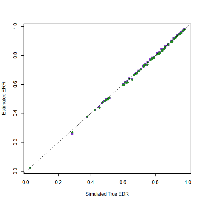
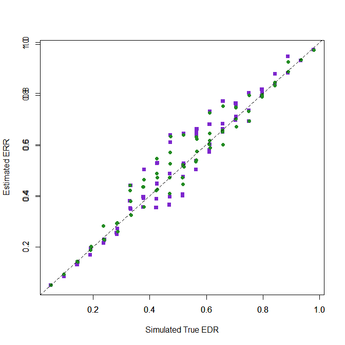
• It has been validated through extensive simulation studies (e.g., Bartoš & Schimmack, 2022).
• It has been applied in high-visibility empirical applications, including analyses of ego depletion, terror management theory, and reproducibility datasets.

If validation is judged only by mathematical proofs, then widely used tools like PET-PEESE, trim-and-fill, and even p-curve should also be excluded. Simulation-based validation is standard for new methods in meta-analysis and remains the most appropriate test of performance under realistic conditions.

6. “Observed z-values are just transformations of p-values, so z-curve is built on ‘problematic inputs’”

This misunderstands the role of observed statistics.

• Z-curve models the distribution of observed z-values under selection, not individual p-values or “observed power.”
• The fact that p-values, z-values, and observed power are monotonic transformations is correct but irrelevant. Z-curve does not interpret individual z-values — it uses their distributional shape to infer the underlying power distribution.

This is exactly how selection models operate.

7. “The authors redefine power unnecessarily”

We do not redefine power. We clarify standard distinctions between:

• True power: based on the true (possibly unknown) effect size
• Observed power: a transformation of the observed test statistic
• Average power: the mean true power across studies in a set

Clarifying these concepts is essential in a literature where the misuse of “post hoc power” is widespread. Reviewer 1’s reference to Lehmann and Romano supports our definitions, not contradicts them.

8. “Confidence intervals around average power are misleading”

This critique misunderstands how confidence intervals behave for bounded parameters like proportions.

Yes, CI width varies depending on the point estimate (e.g., is narrower near 0 or 1, wider near 0.5). That is a general property of binomial-like estimates — not a flaw. The bootstrap method used by z-curve is a standard approach to estimating uncertainty under selection and mixture models.

9. “The coin analogy is flawed”

The analogy is pedagogical, not literal. It illustrates that while we cannot infer the success probability of a single study from one outcome, we can infer the average success probability across a population of studies — just as one might estimate the average fairness of a population of coins.

This mirrors how z-curve infers average power: not by analyzing individual studies in isolation, but by modeling the ensemble.

10. “This work lacks novelty”

Clarification of foundational concepts is a valid scholarly contribution — especially when misunderstanding remains widespread.

• Average power continues to be mischaracterized in the literature.
• Authors such as Pek et al. argue it is invalid to estimate power from completed studies — a position we show to be logically and statistically incorrect.
• Our manuscript synthesizes definitions, clarifies use cases, and corrects misinterpretations.

This is exactly what a commentary should do.

✅ Conclusion

None of the reviewers’ critiques undermine the central argument:

• Average power is a meaningful population parameter.
• It can be validly estimated from published studies using methods like z-curve.
• These estimates are informative about replication, false discovery risk, and the reliability of research literatures.

We stand by the manuscript’s reasoning and hope it will contribute to better understanding in a different venue.

The Action Letter and Reviews

FW: Your Submission MET-2025-0121 – [EMID:1f61f4216ccfe419]

MET-2025-0121
An Average Power Primer: Clarifying Misconceptions about Average Power and Replicability
Psychological Methods

Dear Ms Soto,

I have now received the reviewers’ comments on your manuscript. Based on their analysis and my own evaluation, I can no longer consider this manuscript for publication in Psychological Methods.

Your manuscript certainly touches on an important topic at the intersection of several current methodological research areas of interest to psychologists: power, replication, evaluating research literatures, and study selection. The interest in clarifying areas of confusion is commendable. Despite this, the three reviewers raised several concerns and all three ultimately recommended rejection of the current work. Their comments are thorough, so I will not reiterate them here. I hope they will be helpful to you as you revise this for another outlet.

If I were to make a suggestion in addition to the guidance offered by the reviewers, I might consider a different structure or format for the manuscript. The current submission seemed to be trying to accomplish several different goals: a primer on concepts related to average power, a directed commentary to specific points raised in papers by Pek and McShane, and a demonstration of z-curve – it might be better to focus more. If your goal is to develop a tutorial, I think that the scope would need to be expanded and the language made more precise to increase accessibility given the established earlier work on the topic. For example, the way different types of power are described differs slightly throughout the paper, which may lead to some confusion (see Reviewer 1’s comment on this). While I like that you used a coin example to teach the concept, I would suggest more carefully clarifying how using average observed power differs from using observed power on a single study (e.g. many coins vs 1 coin). Changing the definition of power upfront to focus on significance regardless of the true effect could also use additional clarification. Finally, replication should also be more explicitly defined, particularly in the context of there being multiple options (a few used by the open science framework study you use throughout the paper). Considering the paper as more of a commentary, I understand from your cover letter that you initially considered AMPPS – given that AMPPS specifically encourages commentaries, I might suggest reconsidering AMPPS, taking into account the critiques offered by the reviewers (e.g., considering what is gained by using only an average without considering variability).

For your guidance, I append the reviewers’ comments below and hope they will be useful to you.

Thank you for giving us the opportunity to consider your submission.

Respectfully,

Samantha F. Anderson, Ph.D.
Associate Editor
Psychological Methods

Reviewers’ comments:

Reviewer #1: This commentary has four aims. In particular, as explicitly discussed on page 3 of the introduction, it seeks to:

[1] Clarify the definition of average power.

[2] Argue that point and interval estimate of average power “can be used to assess the credibility of the original results despite uncertainty.”

[3] Provide a case study illustration [2] in the context of data from the terror management literature.

Less explicitly, the commentary also seeks to:

[4] Serve as an apologia for a nascent forensic meta-analytic procedure dubbed “z-curve.”

I will discuss each of these in turn. Before doing so, I note that for the purposes of this review, I will not question the commentary’s focus on “statistical significance” and the purported notion that the goal of a study or replication thereof is to attain “statistical significance.” I disagree with this perspective but that is a different discussion and so I will for the most part adopt the stance of the commentary with regard to this matter.

[1] Definition of Average Power

The commentary defines average power and estimates thereof in a number of places including:

Abstract: “the hypothetical outcome if original researchers had to replicate their studies with new samples.”

Page 3: “[I]f researchers repeated their original studies exactly, using the same methods and sample sizes, how likely would they be to obtain significant results again in a new sample with new sampling error?

Page 5: “estimate the expected success rate if the same study were repeated under identical conditions with a new random sample.”

Page 6-7: “hypothetical prospective replication studies that by definition are identical to the completed studies…The key question is what results one would expect in a hypothetical replication project where the original authors redo their studies exactly as they were done, but with a new sample.”

Page 9: “to wonder how many significant results terror management researchers would find if they redid their studies the same way with new samples.”

Page 16: “Average power is an estimate of the success rate of hypothetical exact replication studies that only differ in sampling error.”

These definitions are more or less correct with the last being the most precise of all because it invokes the notion of differing only with respect to sampling error. Nonetheless, even this definition is not quite correct because it confuses (as does the commentary in general) estimand and estimate.

Recall the following definitions:

– Estimand: Some quantity one wants to estimate (e.g., the average height of women in Spain).

– Estimator: A procedure applied to data that yields an estimate (e.g., the mean is the procedure that sums the data values and divides by the number of them).

– Estimate: The result of applying an estimator to data (e.g., 1.63 meters).

Therefore, I correct the definition given on page 16 to distinguish between estimand and estimate:

“Average power is the success rate of a set of hypothetical exact replication studies that only differ in sampling error. An estimate of average power is an estimate of this success rate.”
[where “success rate” is taken as meaning percentage of the replication studies in the set that yield “statistical significance”]

Importantly, the commentary also says what average power is not in a number of places including:

Abstract: “not to predict the outcome of future replication studies”

Page 3: “the primary purpose of estimating average power is not to predict outcomes of future replication studies”

Page 5: “The goal is not to assign a probability to the set of realized studies with a fixed outcome”

Page 7: “predicting outcomes of new replication studies is not the primary goal of estimating average power”

These all seem correct although I would omit “primary” from the last quotation.

I can see a place for a very short note that clarifies what precisely average power is and what it is not. This is valuable.

However, such a note is not necessary: this has already been done in the second page of the article by McShane, Bockenholt, and Hansen (2020) cited by the commentary (page 186 of that article using the journal page numbers).

[2] Use of Average Power and Estimates Thereof

I do not find average power useful and for a reason that is made abundantly clear by its definition in terms of differing only with respect to sampling error.

Sampling error is a fiction and we cannot repeat studies in a manner such that they “only differ in sampling error” as the definition on page 16 posits.

We are, as the commentary makes clear, in the realm of the hypothetical.

Or, as McShane, Bockenholt, and Hansen put it on their page 186, “average power is relevant to replicability if and only if replication is defined in terms of statistical significance within the classical frequentist repeated sampling framework.” In doing so, they concur that this framework means replication studies that differ only with respect to sampling error and emphasize that that framework is “purely hypothetical and ontologically impossible” (and that replication success need not be defined in terms of “statistical significance”).

Since everyone including the authors of the commentary seem to agree on this, I find it puzzling that the authors find estimates of average power useful and argue that:

Page 3: “average power estimates and their corresponding confidence intervals can be used to assess the credibility of original results despite uncertainty.”

I mean this may be narrowly true in the “purely hypothetical and ontologically impossible” fashion discussed above, but I am not sure what to do with it.

To illustrate this, let’s suppose that I know that the average power of some original set of studies is 50%. In doing so, let’s set aside the notion of estimation uncertainty and suppose that I am correct: average power really is 50% and I know it to be exactly this value.

How am I to use this to evaluate the credibility of a set of original studies even in a purely hypothetical fashion?

I do not think that average number of 50% tells me very much.

It could be that the average is 50% because all of the original studies had 50% power (let’s also set aside the objection about whether it is meaningful speak of the power of a single study) in which case it would seem that studies in this domain should use larger sample sizes.

It could alternatively be that the average is 50% because half of the original studies were “null” and thus rejected 5% of the time and the other half had 95% power, in which case there is some moderator that one needs to identify to distinguish the two.

It could be many, many other things!

Average power simply cannot distinguish among them.

This is why I really enjoyed the authors discussion of coin flips on pages 5-6:

The authors correctly state that based on a single toss of a coin with probability p of heads (0 < p < 1), we cannot infer anything about p. However, based on a single toss each of many coins each with their own probability p_i, we can infer something about the average of the p_i.

However, averages are often not so useful as my 50% example above demonstrates. It is important to also know something about the variation in (or the distribution of) the p_i.

Unfortunately, with only a single flip of each coin, we cannot infer anything about the variation in (or the distribution of) the p_i. Therefore, we cannot distinguish between possibilities such as all 50%, half 5% and half 95%, and others that yield the same average.

To do so, we would need more granular information: we would need multiple flips per coin which we do not have.

[Of course, in the analogy, the coins are studies and a flip determines “statistical (non)significance” and we never get to “flip” a given study more than a single time.]

As a final comment, in the quotation from page 3 given above, the authors discuss the “credibility of original results” and they also elsewhere discuss the “evidential value of published research” (page 1, page 3, page 7). These are ambiguous and undefined terms with no formal meaning in a technical literature. If the authors would like to continue using these terms, it would be helpful if they provided formal definitions. I am left wondering what precisely these vague concepts represent in the authors’ minds.

[3] Application to Terror Management

Given that the authors and I disagree on [2], it will be unsurprising that I do not find this application very compelling. That follows as a logical consequence.

However, I find average power particularly strange in this application. With 852 studies, it seems especially bizarre to me to focus on an average. There must be variation across these studies and known moderators that associate with or “explain” the variation. It seems strange to ignore this valuable additional information.

Also, I strongly disagree with the following claim on page 12:

“The important empirical conclusion is that the data do not rule out the possibility that the entire literature rests on false positive results. The fact that the confidence interval is very wide does not undermine this conclusion because the burden of proof is on researchers who want to provide evidence for their theory.”

This is rather presumptuous: Who are the authors to arrogate to themselves the right to choose on whom the burden of proof lies? Such haughtiness and superciliousness has no place in research, and each person can decide for himself or herself on whom to place the burden of proof.

Indeed, Neyman was quite clear when elaborating his decision theory that there was subjectivity involved in choosing which of two hypotheses would be the tested one and which would be the alternative one. He emphasized that two different people could have different perspectives and one person might reasonably choose one of the two hypotheses to be the tested hypothesis while the other person might reasonably choose the other of the two hypotheses to be the tested hypotheses (see, for example, page 106 of Neyman (1977), “Frequentist probability and frequentist statistics,” Synthese).

The authors also make a confusing statement on page 14 when they write “if all studies had an average power of 10%, selection for significance could not select for more powerful studies.” As mentioned above, it is not clear whether it is meaningful to speak of the power of a single study. However, it is certainly not meaningful to speak of the average power of a single study as in this quotation. What are you getting at here? The average of a single value is the value itself and so it is not meaningful to talk of an average of a single value as you appear to be doing here.

Finally, as discussed in greater details below, this application moves beyond average power and so all parts of the application that do so are not germane to an “Average Power Primer” commentary. Please remain firmly focused on average power.

[4] Apologia pro z-curve

This commentary is about the concept of average power. It is not the place to showcase let alone mount a full-throttled endorsement of a method that could at best be described as “emerging.” The z-curve is a new and unproven method. The papers introducing it are light on mathematical statistics. They instead make heavy use of analogy and metaphor and they use small numbers of (arguably questionably-parameterized) simulation studies to make rather broad and sweeping claims. Simulation studies are no substitute for mathematical statistics and are constrained by the creativity of the simulator as well as the motivation of the simulator to make a method look good or bad. Like all methods, the z-curve requires deep formal investigation before it is ready for the wild.

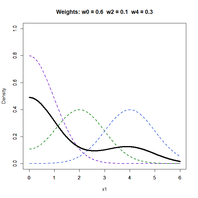
Another problem with ad hoc, improvised “emerging” methods like the z-curve is that they are a moving target. For example, should there be three unspecified components estimated along with their weights by minimizing the sum of the squared distance of a kernel density estimate and a theoretical quantity as in the z-curve of Brunner and Schimmack 2020? Should there be seven pre-specified components (at 0, 1, 2, 3, 4, 5, and 6) with weights estimated by maximum likelihood via the expectation-maximization algorithm as in the z-curve of Bartos and Schimmack 2022? Should it be whatever Schimmack and colleagues (or for that matter someone else) decide it should be at some future date? It is hard to know: the method is still under development and refinement and we should cautiously step back until it is fully baked.

Another reason the z-curve is out of place in a commentary on average power is that the purpose of the z-curve is not to estimate average power. Instead, the purpose of the z-curve is to estimate the distribution of power (the estimate of the average and other quantities is simply a byproduct of estimating the distribution).

Therefore, the wonderful coin flip analogy that the authors provide on pages 5-6 does not apply to the z-curve because the z-curve does not make use of a binary input (was the original study “statistically significant” or not) but rather makes use of a more granular continuous input (what was the observed power of the original study).

The current authors write on page 5 that observed power of single study is “problematic”. It is unclear why they think that a method that takes in a bunch of “problematic” inputs like the z-curve can somehow launder them and provide something of value.

If your response is that the z-curve takes as input observed z-statistics rather than observed power, this may be technically true but it is not a relevant objection: observed z-statistics, observed p-values, and observed power are all one-to-one transformations of one another so it all amounts to the same thing.

More focused comments:

1. Page 4: The authors redefine power, which is rather curious. It also seems unnecessary. Regardless, in doing so, they mix up concepts from Neyman-Pearson decision theory. When the tested hypothesis and alternative hypothesis are both simple point hypotheses, power refers to a probability under the alternative. However, once either the tested or alternative is composite, we no longer talk of power in that way. Instead, we simply talk of the power function where one of the input parameters to the power function, which I will denote theta (consistent with the commenatary authors), takes any value in the space Theta regardless of whether that value belongs to the partition being tested or to the alternative. See any mathematical statistics texts for this, although I would point to Chapter 3 of Lehmann and Romano (page 57):

“The probability of rejection (3.2) evaluated for a given θ in Ω_K is called the power of the test against the alternative θ. Considered as a function of θ for all θ ∈ Ω, the probability (3.2) is called the power function of the test and is denoted by β(θ).”

There is hus no need to redefine power or discuss conditional versus unconditional power or any of this.

2. Page 4: After distinguishing among hypothetical power, observed power, and true power, the authors write “We refrain from the use of terms such as a prior and post-hoc power because power calculations can be conducted before and after a study, and power calculations after a study can use hypothetical values or observed data.”

I find this a bit weasily or overly rhetorical or something. Specifically, with regard to the schema the authors introduce:

– Hypothetical power can be evaluated a priori or post hoc.

– Observed power is necessarily post hoc

– True power is simply not relevant because it is never known (whether a priori or post hoc)

Average power is simply an average of post hoc powers (filtered through—of course and as always—some model for the data).

Also, given that the authors seem to abandon this schema right after introducing it, I am not sure that they need introduce it in the first place.

3. Page 5: You criticize Pek here and throughout but I am not sure it is so on the mark. For instance, consider the following from page 364 of Greenland (especially the bit about the horses):

“Among the problems with power computed from completed studies are these:
1. Irrelevance: Power refers only to future studies done on populations that look exactly like our sample with respect to the estimates from the sample used in the power calculation; for a study as completed (observed), it is analogous to giving odds on a horse race after seeing the outcome.
2. Arbitrariness: There is no convention governing the free parameters (parameters that must be specified by the analyst) in power calculations beyond the alpha-level.
3. Opacity: Power is more counterintuitive to interpret correctly than P values and confidence limits. In particular, high power plus ‘nonsignificance’ does not imply that the data or evidence favors the null (6).”

Greenland (2012), “Nonsignificance Plus High Power Does Not Imply Support for the Null Over the Alternative.” Annals of Epidemiology.

4. Page 5, Page 8, etc.: You frequently label power a parameter or liken it unto one. Power is not a parameter or akin to one!

5. Page 10: Why did Chen only code |z| > 1.96 studies? Can you elaborate? This seems like a poor choice.

6. Page 12: You write “Power is limited by alpha and cannot be less than 5%.” This is not the case. See, for example, Chapter 4 of Lehmann and Romano.

7. Page 14: What is “zing”?



Reviewer #2: The manuscript “An average power primer: Clarifying misconceptions about average power and replicability” (MET-2025-121) engages with the perspectives presented by McShane et al. (2020) and Pek et al. (2024). The authors forward that: (a) using observed data to estimate true power to evaluate the credibility of published studies does not constitute an ontological error and (b) high uncertainty of an estimate does not negate its diagnostic value.

The manuscript forwards the use of computing average power with the Z-curve, but certain aspects of the interpretation of average power could benefit from additional clarification to mitigate potential ontological misunderstandings. Furthermore, the concepts of “credibility” and “evidentiary value,” although associated with average power, currently lack formal definitions, which may impact their interpretability. Lastly, the rationale for maintaining the diagnostic relevance of estimates with high uncertainty would be strengthened by elaboration. Below, we expand on the points, seeking more clarity on the author(s)’s position while pointing to relevant findings by McShane et al. (2020).

ONTOLOGICAL ERROR. An ontological error occurs when power is improperly ascribed to in a way that does not align with its natural (ontological status). Classical power quantifies the pre-data performance of a study/design/procedure/test over hypothetical random data. Throughout, we use the term test in place of study/design/procedure/test. Average power (i.e., the average of a population of heterogeneous tests) also quantifies test performance over hypothetical random data. An ontological error occurs when the probability of power over random data (i.e., in the context of pre-data) is interpreted as a post-data probability (i.e., applied to fixed/observed data).

The authors recognize the ontological error in the following statements:
p. 5: “We also do not discuss the problematic use of observed power to evaluate the results of a single study (Hoenig & Heisey, 2001).”

p. 5: “The goal is not to assign a probability to a set of realized studies with a fixed outcome, but to estimate the expected success rate if the same study were repeated under identical conditions with a new random sample.”

However, some instances of vague phrasing could potentially be misinterpreted in a way that suggests an ontological error, where the pre-data concept of power might appear to be applied post-data.

The following phrases may unintentionally contribute to this misunderstanding.

p. 4 – 5: “…power calculations after a study can use hypothetical values or observed data.” It would be helpful to clarify whether these calculations are interpreted as pre-data power or have a post-data interpretation.

p. 6: “… the long run probability of studies to produce the observed outcome.” It is unclear in this statement whether power is treated as a pre-data concept or a post-data concept (i.e., observed power).

p. 7: The following sentence, “Taken at face value, this finding implies that studies had an average power of 97%” could be made clearer by being specific about whether power is applied to pre-data or post-data studies.

Perhaps helpful distinction to make would be the difference between average (pre-data) power versus average observed power, in which the later (like observed power) is a transformation of the p-value
as described in Hoenig & Heisey (2001).

CREDIBILITY AND EVIDENTIARY VALUE. On p. 3, the authors state “We clarify that the primary purpose of estimating average power is not to predict outcomes of future replication studies, but to evaluate the credibility of the published studies by estimating their true average power.” Later, on p. 7, they further explain: “Estimates of average power, however, make it possible to distinguish credible results that were driven by true effect sizes from sets of studies with low average power that may contain a large percentage of false positive results (Sorić, 1989).” The term “credibility” is referenced throughout the manuscript but has not been formally defined, leaving room for multiple interpretations. Clarification on how pre-data average power or average observed power are conceptually linked to credibility would help ensure a more precise understanding of its application. A clarification of “true power” and how it helps distinguish “credible results” would also strengthen the argument.
Additionally, on p. 7, the authors write: “In short, average power estimation provides a diagnostic tool for evaluating the evidential value of sets of studies.” Similar to the term “credibility,” the term “evidential value” has not been explicitly defined. A more detailed explanation of this concept in relation to pre-data average power and credibility would enhance interpretability.

UNCERTAINTY. Including more information in terms of multiple tests in average power might decrease uncertainty in estimation (shown by McShane et al. 2020). In average power, there are two sources of uncertainty in its hierarchical setup in which tests are nested within a population of tests. Sampling variability is termed epistemic uncertainty in that it is reduced by increasing the number of sampling units (i.e., tests). However, between-test variability does not decrease with increasing the number of tests. This kind of uncertainty is called aleatory uncertainty. When more tests are sampled, the average power estimate becomes more precise with diminishing sampling variability but the distribution representing the heterogeneity between tests (aleatory uncertainty) is better estimated. A key point to consider is whether the average is a good summary statistic of a heterogenous population. Heterogenous populations might have multiple modes, a skewed or even a uniform distribution. It would help to clarify when the mean is a reasonable summary of a heterogenous distribution.

Furthermore, McShane et al.’s (2020) concern about uncertainty is that the width of the CIs about average power depends on the corresponding point estimate of average power. Thus, tight CIs will be obtained at low and high estimated values of average power, and large CIs will be observed at estimates of average power close to .50. As stated by McShane et al. (2020), a narrow CI does not purely indicate estimate precision, but that the estimated average power is close to its theoretical bounds; in contrast, a wide CI would indicate that the average power estimate is close to .50. The CIs are inherently tied to the point estimate and do not serve as an independent measure of estimate precision. Thus, they cannot be interpreted as such.

Minor points:
The definition used in the manuscript – specifically, requiring p < .05 twice for similarly implemented studies (cf. Open Science Collaboration, 2015) is relatively narrow. Several methodologists (e.g., Anderson & Maxwell, 2016; Fabrigar & Wegener, 2016, 2017; Fife & Rodgers, 2021) have raised concerns about the limitations of this definition and have proposed alternative perspectives on replication. Acknowledging these differing viewpoints would provide a more comprehensive discussion an enhance the manuscript’s engagement with the broader literature on replication. Additionally, Gigerenzer (2018) has critiqued the emphasis on statistical significance (cf. the concept of power), characterizing it as a ritual that might lead to misconceptions. Considering this critique, as well as similar points raised by McShane et al. (2020), further discussion on how the author(s)’ perspective aligns with or diverges from these concerns could be valuable. How might the author(s)’ perspective on replication address these other points made by the discipline?

p. 7: Define “false positive risk.”

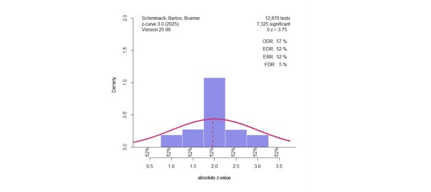
A technical issue: The EDR has a CI with a lower limit of 0.05. If one were to use this CI to conduct a hypothesis test, H_0: EDR = 0.05 (not one-sided) cannot be rejected. Because 0.05 is the lowest possible EDR, EDR = 0.05 implies that the distribution of the noncentrality is concentrated at a single value of zero. However, ERR has a CI whose lower limit is 0.12. This is contradictory because a zero non-centrality means the ERR should be 0.05 (or even lower if directional). The reason for this inconsistency is likely due to bootstrapping the CI, which may not be technically sound near a parameter boundary.

p. 7: “selection bias systematically inflates the observed success rate.” This statement makes an untestable assumption that selection bias only decreases the publication rate of insignificant results. However, it is also possible that the publication rate for significant results is also imperfect.
For example, if the true EDR is 0.6, which can be written as 0.6 = 0.6 * 1 / (0.6 * 1 + 0.4 * 1) without any publication bias. Suppose that the publication rate for significant studies is 0.5 and that for insignificant studies is 0.6, then the ODR is 0.6 * 0.5 / (0.6 * 0.5 + 0.4 * 0.6) = 0.56 < 0.6.
So, for ODR to be less than EDR, it seems that we need to assume that the selection function is monotone (more likely to select significant studies for publication than insignificant ones).

p. 8: “From this finding, we can also infer that effect size estimates are likely inflated because the true population effect size would not produce a significant result. This conclusion is implied by the statistical fact that a p-value equal to alpha (.05) corresponds to 50% power.” These statements could benefit from additional clarification. The true effect size and power are population quantities whereas statistical significance and p-values pertain to sample quantities. Given this distinction, further explanation of how a direct correspondence between the two is established would enhance the clarity of the argument.

p. 8: The phrase “observed parameters” seems contradictory. Parameters are often used to describe population values that are unobserved. And observed estimates are used to describe statistics calculating using sample data (which are estimates of population parameters).

p.2: The authors claim that the Z-curve is based on solid mathematical foundations and has been validated with extensive simulation studies. The inferential targets of Z-curve (EDR, ERR, and FDR) could be more carefully examined because analytics and the reported simulations do not consider potential violations of model assumptions in empirical data (e.g., how publication bias occurs; see MacCallum, 2003 on working with imperfect models). It is unlikely that these model assumptions match empirical data, and it remains to be examined how Z-curve performs under less-than-optimal conditions that could better reflect reality.

The development of the Z-curve might be better contextualized with related forensic meta-analytic procedures, which are designed for assessing the quality of the evidence in a set of results (Morey & Davis-Stober, under review). There is much discussion on the usefulness of such forensic methods (e.g., Gelman & O’Rourke, 2014), and it would be helpful to readers to provide a review of this literature. Papers on related forensic meta-analytic procedures are by Morey (2013), Pek et al. (2022), Bishop and Thompson (2016), Erdfelder and Heck (2019), Montoya, Kershaw, and Jergens (2024), and Ulrich and Miller, 2018).

p. 12: The author(s) report a range of possible false discovery risk (FDR) values from .26 to 1.0. It is important to recognize that the FDR is an upper bound to the false finding rate (FFR; Ioannidis, 2005; Pashler & Harris, 2012). However, further clarification is needed to determine whether FDR functions as a tight upper bound to FFR. Additionally, the statement “FDR of 100% creates reasonable doubt about the credibility of evidence” may benefit from more nuanced wording. Since 100% is an upper bound of any lower value, including 0%, the actual FFR remains uncertain based solely on information about the FDR. Given this uncertainty, it may be more prudent to interpret the lower bound of the FDR cautiously when assessing the likelihood of false findings.

==
Anderson, S. F., & Maxwell, S. E. (2016). There’s More Than One Way to Conduct a Replication Study: Beyond Statistical Significance. Psychological Methods, 21, 1-12. https://doi.org/10.1037/met0000051

Bishop, D. V., & Thompson, P. A. (2016). Problems in using p-curve analysis and text-mining to detect rate of p-hacking and evidential value. PeerJ, 4, e1715. https://doi.org/10.7287/peerj.preprints.1266v4

Erdfelder, E., & Heck, D. W. (2019). Detecting evidential value and p-hacking with the p-curve tool. Zeitschrift Für Psychologie, 227(4), 249-260. https://doi.org/10.1027/2151-2604/a000383

Fabrigar, L. R., & Wegener, D. T. (2016). Conceptualizing and evaluating the replication of research results. Journal of Experimental Social Psychology, 66, 68-80. https://doi.org/10.1016/j.jesp.2015.07.009

Fabrigar, L. R., & Wegener, D. T. (2017). Further considerations on conceptualizing and evaluating the replication of research results. Journal of Experimental Social Psychology, 69, 241-243. https://doi.org/10.1016/j.jesp.2016.09.003

Fife, D. A., & Rodgers, J. L. (2021). Understanding the exploratory/confirmatory data analysis continuum: Moving beyond the “replication crisis”. American Psychologist. https://doi.org/10.1037/amp0000886

Gelman, A., & O’Rourke, K. (2014). Discussion: Difficulties in making inferences about scientific truth from distributions of published p-values. Biostatistics, 15(1), 18-23. https://doi.org/10.1093/biostatistics/kxt034

Gigerenzer, G. (2018). Statistical Rituals: The Replication Delusion and How We Got There. Advances in Methods and Practices in Psychological Science, 1(2), 198-218. https://doi.org/10.1177/2515245918771329

Hoenig, J. M., & Heisey, D. M. (2001). The abuse of power: The pervasive fallacy of power calculations for data analysis. The American Statistician, 55(1), 19-24. https://doi.org/10.1198/000313001300339897

Ioannidis, J. P. (2005). Why most published research findings are false. PLoS: Medicine, 2(8), e124. https://doi.org/10.1371/journal.pmed.0020124

MacCallum, R. C. (2003). 2001 presidential address: Working with imperfect models. Multivariate Behavioral Research, 38(1), 113-139. https://doi.org/10.1207/S15327906MBR3801_5

McShane, B. B., Böckenholt, U., & Hansen, K. T. (2020). Average Power: A Cautionary Note. Advances in Methods and Practices in Psychological Science, 3(2), 185-199. https://doi.org/10.1177/2515245920902370

Montoya, R. M., Kershaw, C., & Jurgens, C. T. (2024). The inconsistency of p-curve: Testing its reliability using the power pose and HPA debates. PloS ONE, 19(7), e0305193. https://doi.org/10.1371/journal.pone.0305193

Morey, R. D. (2013). The consistency test does not-and cannot-deliver what is advertised: A comment on Francis (2013). Journal of Mathematical Psychology, 57(5), 180-183. https://doi.org/10.1016/j.jmp.2013.03.004

Morey, R. D., & Davis-Stober, C. P. (2024). On the poor statistical properties of the p-curve meta-analytic procedure. Unpublished manuscript, School of Psychology, Cardiff University, Cardiff, United Kingdom.

Open Science Collaboration (2015). Estimating the reproducibility of psychological science. Science, 349, aac4716. https://doi.org/10.1126/science.aac4716

Pashler, H., & Harris, C. R. (2012). Is the replicability crisis overblown? Three arguments examined. Perspectives on Psychological Science, 7(6), 531-536. https://doi.org/10.1177/1745691612463401

Pek, J., Hoisington-Shaw, K. J., & Wegener, D. T. (2022). Avoiding Questionable Research Practices Surrounding Statistical Power Analysis. In W. O’Donohue, A. Masuda, & S. Lilienfeld (Eds.), Avoiding Questionable Practices in Applied Psychology(pp. 243-267). Springer. https://doi.org/10.1007/978-3-031-04968-2_11

Pek, J., Hoisington-Shaw, K. J., & Wegener, D. T. (2024). Uses of uncertain statistical power: Designing future studies, not evaluating completed studies. Psychological Methods. https://doi.org/10.1037/met0000577

Sorić, B. (1989). Statistical “discoveries” and effect-size estimation. Journal of the American Statistical Association, 84(406), 608-610. https://doi.org/10.1080/01621459.1989.10478811

Ulrich, R., & Miller, J. (2018). Some properties of p-curves, with an application to gradual publication bias. Psychological Methods, 23(3), 546-560. https://doi.org/10.1037/met0000125





Reviewer #3: An Average Power Primer: Clarifying Misconceptions about Average Power and Replicability

This is an interesting paper that leverages published work and an R package (and an alternative) that aims to help understand replication success from average power. The ideas are not original here but in prior work. The context is important. The article is aimed to address issues with this general approach that others have downplayed and for which the authors espouse, citing recent literature on the topic.

The manuscript (ms.) discusses replication studies and their importance, but is itself doing something different (via average power of published studies). My understanding from recent work is that the power of an original study is calculated differently than the power of a replication. There are corrections. For example, in this journal Anderson and Kelley have essentially a treatise on study design for replication, both from a power and an accurate perspective. They make clear why the power of a replication – where publication bias is very likely to occur – needs to be done differently. Thus, replication studies should not be planned like original studies, which I think the authors here would agree with. Work by Anderson and colleagues also provide methods for actually doing this planning. This involves using methods in which a maximum likelihood estimate of the true parameter is found and used for study design. The authors here are not doing that, per se, but they are trying to back into power of the research area from the studies. I think this is easier said than done and the necessary assumptions are not well specified nor are they reasonable, in the sense that a researcher planning a study is in a particular context whereas the collection of published studies in an area will be from multiple contexts, populations, various treatment effect sizes, etc.

The use of power or sample size planning more generally clearly has many advantages in original research. As well as when planning replications. But there are multiple ways of thinking about sample size planning. And there are multiple ways of thinking about power, even if the average power from a given area is worth estimating (realizing each study is not an exact replication itself).

The authors say “We clarify that the primary purpose of
estimating average power is not to predict outcomes of future replication studies, but to evaluate the credibility of the published studies by estimating their true average power.” Calling into question the credibility of a corpus of studies from an area because the average power is low would be akin to calling into question the health of individuals writ large in a city in which the average health is not good. Of course the average is useful, but it misses important things (namely the various upper percentiles). I am not even sure if we need “true average power” as studies tend to differ on various dimensions. Average power says nothing about the most properly conduced and planned studies. Sure, we can average over all of that, but that doesn’t address either (a) how to plan an original study or (b) how to plan a replication study. It also would not be good to talk about the replication effectiveness of an entire area because of the average power in published research. If few studies are exact replications, does the average power of them even make sense?

The authors say “if researchers repeated their original studies exactly, using the same methods and sample sizes, how likely would they be to obtain significant results again in a new sample with new sampling error?” Well, it depends on if the original studies are those that are simply finished or if it is for those that are published (and have significant findings). Average power of significant findings that are published is clearly not the same as average power for all studies ever conducted on the topic (not withstanding the point about stepping into the same river twice, which maybe can or maybe cannot be done; McShane and Bockenholt, this journal).

Design considerations beyond power would strengthen the manuscript. The z-curve work is not new here. Psychological Methods is not the place for illustrating new methods, generally speaking.

The authors define power as “We therefore define power ( ) as the unconditional
probability of producing a significant result (Bartoš & Schimmack, 2022).” But power depends on the null hypothesis being false (definitionally). They state that “The conditioning on a non-zero effect size makes sense for a priori power analysis, but it cannot be applied to estimates of true power because some studies may have population effect sizes of zero.” To the extent that the idea they are after should be quantified, then the power that they reference should be “average power” but not “power.” As different studies will consist of different populations and different contexts, mixing multiple theoretically different values of power to have an average is limited, at best. They go on to define three types of power, which is somewhat useful but also they get into a confusing set of terms. A table would be useful here.

Regarding the replication project and post hoc power, the authors state that “The goal is not to assign a probability to the set of realized studies with a fixed outcome, but to estimate the expected success rate if the same study were repeated under identical conditions with a new random sample.” But to do this, one needs more than just the p-value of the obtained study of interest. It is not the same as estimating the true proportion of a binary outcome because of publication bias.

The coin example is not good because, again, conditional probability is important. In that sense, if the type I error is true, the probability of rejecting the null is 5% (or alpha more generally). But if the specified parameter setting and assumptions are satisfied, etc., 50% power does mean that it would be like a coin flip. But, only in this conditional situation; not only the null false, but false to the tune exactly specified in the power analysis.

The authors might benefit from discussing what is meant more about the ontological error.

The authors state: “he original studies used for the Reproducibility Project had a 97% success rate (Open Science Collaboration, 2015). Taken at face value, this finding implies that the studies had an average power of 97%. ” But I do not agree with this. This statement needs to be nuanced considerably. The issue is that there is a selection effect; and selection effects change meanings. The published studies were in part selected (if not wholly selected) due to the significant finding.

The authors aim to “argue that the primary purpose of average power estimation is not to predict the outcome of future replication studies, but the hypothetical outcome if original researchers had to replicate their studies with new samples.” But I disagree with this. Average power is only getting at the mean power (unconditionally as no covariates are used) of published studies in the literature.

The authors seek to “clarify that the primary purpose of estimating average power is not to predict outcomes of future replication studies, but to evaluate the credibility of the published studies by estimating their true average power.” But consider only a single study is done and published. How does this help us? How many studies of exactly the same scenario need to exist in order to have something reasonable to say? As most published studies (all?) are in some way different (population, age, treatment, time, context, etc.), averaging studies for power and then making an assessment about credibility is filled with potential issues and nuances.

The authors have done published work on this topic already. Other than the terror research findings, which are more aptly described in that literature or only used for an example (as is the case here), I do not find the manuscript to be contributing new information to the Psychological Methods readership. I am sympathetic with the sentiment of Pek et al. (2024) regarding post hoc power. In any instance we have a single draw from some hypothetical distribution. And to the extent to which a study is held exactly constant, we could learn something from many more draws from that study. Of course, one could attempt a meta analysis, too. But regardless, I do not find that there is enough here for the Psychological Readership.

Meta-science is not some special science or Über-science. It works just like other science, and in psychology it means that it is not working very well. The biggest problem is that theoretical or statistically oriented research means are subject to the same capitalistic pressure to produce output that can be measured and contributes to GDP by selling their work to publishers, who earn profits, which makes research workers work at least economically valuable. I mean, most of have tenure and could spend the time we are not doing our paid job (teaching) to go sailing, play tennis, but for some reason, some engage in meaningless pseud-scientific work and flood scientific journals with garbage and waste other people’s time to read their garbage instead of playing tennis. In sort, I am frustrated, and here is why.

I am looking for articles that discuss Vevea’s random effects selection model implemented in the r-package weightr. This summer I found that this is the best way to conduct effect -size meta-analyses in psychology because it models heterogeneity in effect sizes across conceptual replication studies and models selection bias that is pretty much always present in psychology.

This is how I found the article “Effect Size Estimation From t-Statistics in the Presence of
Publication Bias” by Ulrich, Miller, and Erdfelder. I once contacted Ulrich about z-curve, but he was not intersted. Erdfelder was behind G*Power and deserves credit for this free program that helped me to understand power back in 2013.

The article is a long and boring review of different methods to correct for publication bias in effect size estimation. The main point of this review is only to conclude that they all suck and that this is the reason why they developed their own model.

“In sum, all of these approaches are either highly complex or make strong and somewhat implausible assumptions about the weight functions, thus calling for an alternative approach that is based on weaker and more flexible assumptions but still relies on a simple selection model with clear-cut interpretations of the parameters. This motivated our own approach presented in the following section”

Then follows a long introduction of their model with lots of formulas and figures that make it look really, really scientific, and probably scared the shit out of the reviewers at “Zeitschrift für Psychologie,” where this nonsense was published after it was probably rejected from serious method journals.

The “new” model is a simple fixed effects model that assumes all studies have the same population effect size. This makes the model as useless as p-curve or p-uniform the analysis of most real datasets in psychology that typically have a high amount of heterogeneity. Any article with headings like “Maximum Likelihood Estimation of True Effect Size” is not worse reading because there is no True Effect Size in psychology. The only scenario that works well for a fixed effects model is a set of studies where all studies have no effect and significant results were obtained with p-hacking. When there are real effects, they are not all the same across studies. At a minimum, a test of heterogeneity should be conducted before a fixed-effects model is used.

To show how good their new method is, they apply it to a meta-analysis by Shanks et al. 2015) of priming studies. Priming studies are prime candidates for finding no effect and a lot of p-hacking. Their new, super-duper, so much better model estimated a TRUE EFFECT SIZE of d = .44, 95%CI = .31 to .57. Wow, priming works. We were all wrong and should apologize to Bargh. Maybe Einstein primes also make people really smarter. Where is the barf emoji in wordpress?

Of course, they do not compare the result to other methods, which is often recommended because “no method works well in all circumstances,” (Carter et al., 2018), but hey their review showed the other methods suck, so why bother. Fortunately, the Shanks data are openly available (really open data sharing is the best that has come out of the replication crisis), and I can present the results.

Let’s start with the default random-effects selection model implemented in weightr. This model is called the 3PSM model because it has 3 parameters to estimate selection bias at p < .05 (two-sided), the mean and standard deviation of the population effect sizes (i.e., without sampling error).

There is surprisingly little heterogeneity. The standard deviation of effect sizes is estimated to be .09. Thus, 95% of effect sizes are assumed to be either .2 standard deviations above or below the mean. The mean is estimated at d = .44. Thus, the 95%CI is d = .33 to .55. Maybe that is why Ulrich and co did not report model comparisons. Who needs a new model if the old model works just fine. No publication. Where is the crying face emoji?

But it gets better. Many of the non-significant effect sizes are marginally significant and were reported as evidence against the null-hypothesis. We can model this with the random effects selection model by adding a step at p = .05 (p = .10, two-sided is typically the upper value to get away with marginal significance). Indeed, 8 non-significant results are marginal and only 2 are not, because they are marginally-marginally significant. With a small dataset it is difficult to estimate multiple parameters. One way to deal with marginally significant results, would be to fit the model only to “significant” results. Another one is to lower the significance criterion to treat marginal results as significant. All p-values were below p = .14, two-sided. So, I set the significance criterion to .14. In this model, the mean was d = .27, 95% CI = .18 to .36. Using only the results with p-values below .025 (one-sided) produced an estimate of d = .33, 95%CI = .22 to .44.

In short, the article fails to show that the new model is needed or better than previous models. In fact, it is worse because it does not estimate heterogeneity in effect sizes. This is not a major problem for the application to Shank’s priming data, but it would be a problem for other meta-analyses. Using a fixed effect size model with heterogenous data is scientific malpractice and leads to the wrong conclusions.

But what do we do with priming? Should we really believe that priming works in these studies? How robust are these results? Could they be replicated. With most sample sizes below N = 100, effect sizes in a single study are inflated and correction models can do only so much to estimate the true values.

Another way to look at these data is to use z-curve. Being generous, we simply compute the ratio of effect sizes over sampling error and use the t-values as if they were z-values. This produces an upward bias in studies with small samples.

Z-curve makes it clear that non-significant results (left side of 1.96) are clustered just below the criterion for significance. Treating these observations as honestly reported non-significant results would be a mistake and create upward bias in effect size estimates. It also shows that most significant values are clustered close to the value for significance. This suggests p-hacking. Based on this distribution of effect sizes, the model assumes that many more priming studies were conducted, but not reported because they failed to show support for priming. The expected discovery rate of all studies would be only 18% significant results, but this estimate is uncertain and it could be as many as 29% or as little as 5%. Because 5% is expected by chance alone, the false positive risk is 100%. That is, we cannot rule out that all of these results were obtained without a real effect, which is not implausible when we look at priming studies.

The local power estimates below the x-axis also show that even studies with a z-value of 3 (observed power > 80%) have only 24% power to show a significant effect again. The only studies worthwhile to follow up on are 3 results with z > 4, but I would not bet money on these results to replicate successfully. After all, it is priming research.

Ok, now it is time to go and play tennis and have some fun. I am not getting paid enough to spend more time on this shit, but maybe somewhere I can save some people from wasting time on this article or other articles by authors with such a low degree of trustworthiness. If you care about effect–size meta-analysis, read some tutorials on weightr. It is the best program we have so far.

It is widely recognized that no single study is conclusive. Credible evidence requires successful replications by independent researchers (Cohen, 1994). The credibility crisis in psychology has revealed that many hypothesis tests lack robust support for two reasons. First, direct replication studies are rare because they are difficult to publish. Journals have a strong bias to publish new findings rather than reporting that a finding can be successfully replicated. Second, journals have a strong bias in favor of statistically significant results. Thus, it is also hard to publish replication failures with a non-significant result. As a result, psychology journals mostly publish new discoveries supported by statistically significant results, p < .05.

Statisticians have long noted that selective reporting of significant results undermines the credibility of significance testing (Sterling, 1959). When only significant findings are published, statistical significance loses its ability to distinguish between true and false claims. Under such conditions, even implausible results—like time-reversed causality—can appear credible (Bem, 2011). By the early 2010s, researchers recognized that more than half of published findings might be false positives (Simmons, Nelson, & Simonsohn, 2011). This realization helped trigger psychology’s replication crisis. As psychologists began conducting and reporting direct replications, the success rate proved to be alarmingly low (Open Science Collaboration, 2015).

One reason it took so long to recognize psychology’s replication problem is that meta-analyses suggested false positives were rare and that replication failures were mostly false negatives caused by low statistical power. A meta-analysis in the prestigious journal Psychological Bulletin even suggested that paranormal phenomena are real (Bem & Honorton, 1994). During the credibility crisis, it became clear that many meta-analytic findings are unreliable because publication bias inflates the combined effect size estimates. To address this issue, researchers have developed statistical methods that adjust for publication bias (see Carter et al., 2019 for an overview of methods). These methods sometimes reveal that the corrected effect size is not statistically significant, implying that the true effect may be zero (Carter et al., 2019; Meier et al., 2022).

While bias correction is an important improvement, these methods often overlook another major issue: the studies included in psychological meta-analyses are rarely direct replications. Instead, they are typically conceptual replications, varying in procedures and dependent variables. As a result, it is likely that the true effect sizes differ across studies. Indeed, when tested, many meta-analyses reveal substantial heterogeneity (Mertens et al., 2022), yet this variability is often ignored in interpreting results.

In this paper, I present four examples showing how conclusions based on the average effect size change when heterogeneity is taken into account. These examples also serve as a tutorial for investigating heterogeneity in meta-analyses and offer guidance for reanalyzing existing work and conducting more meaningful meta-analyses in the future.

A Brief Introduction to Meta-Analysis

Meta-analyses are used to combine the results of multiple studies to obtain better estimates of population effect sizes. For example, original studies often have low statistical power to reject false null hypothesis with small effect sizes. Combining the results of several studies with low power creates a single dataset with high statistical power. For example, after 10 studies with N = 40 participants have been published, a fixed effect meta-analysis has the power of a single study with N = 400 participants (Schimmack, 2012).

Meta-analyses work well when (a) studies are sufficiently similar so that all studies have similar population effect sizes, and (b) there is no bias in the reporting of results. A good example are the Cochrane reports in medicine (Higgins et al., 2023). Cochrane reports use only studies that test the same treatment on the same outcome. Surprisingly, they also show no sign of publication bias. As a result, a fixed effects meta-analysis of these studies solves the problem of low power in clinical trials and provides useful estimates of the true treatment effect.

In contrast, the application of standard meta-analysis to psychological results ignores that psychological studies are rarely direct replications. To solve this problem, psychologists started using random-effects meta-analysis (Hedges & Vevea, 1998). However, the use of a random effects model did not substantially alter the interpretation of meta-analyses. The main focus remained on the estimate of the average effect size. Another problem is that the standard random effects model does not take publication bias into account and produces inflated estimates when bias is present (Carter et al., 2019).

The problem of methods that correct for bias is that they are essentially fixed-effect size methods. That is, they estimate a single effect size and do not estimate heterogeneity of effect sizes. Thus, meta-analysts have to choose between methods that estimate heterogeneity or methods that correct for bias. This creates problems when these models show evidence of heterogeneity and bias (Mertens et al., 2022). Fortunately, there is one method that can estimate bias, correct for bias, and estimate heterogeneity (Carter et al., 201; Hedges & Vevea, 1996). These models are known as random effects selection models (RESM). However, the model was difficult to implement, and a user-friendly R-package was only published in 2016 (Coburn et al., 2019. Unfortunately, tutorials and applications of the RESM continue to focus on the average effect size estimate and ignore the estimate of heterogeneity (Carter et al., 2019; Meier, VanderWeele, & Mathur, 2022). Here I show how information about heterogeneity in effect sizes can be interpreted and why it is misleading to focus on the average effect size to interpret meta-analyses of conceptual replication studies.

A Simulation of Heterogeneity and Selection Bias with an Average Effect Size of Zero

Carter et al. (2019) used simulation studies to evaluate the performance of several meta-analytic methods, including the RESM. They used an RESM with three parameters (3PSM). The first parameter estimates the average effect size. The second one estimates heterogeneity, and the third one estimates the amount of bias in reporting of non-significant results.

The simulation study simulated standardized effect sizes for between-group differences (Cohen’s d). I focus on the simulation with high heterogeneity because it is most similar to meta-analyses of conceptual replication studies. The simulation assumes that population effect sizes have a normal distribution with a mean of 0.0 and a standard deviation of 0.4 (Figure 1).

Figure 1 also shows the distribution of the effect size estimates in 5,000 simulated studies using Carter et al.’s (2019) simulation of high selection bias and no p-hacking. The distribution is shifted towards positive results. The small pump of negative results is due to the simulations weaker bias against significant negative results. All of the negative results are statistically significant.

Carter et al. (2019) fitted the three parameters selection model (3PSM) to these data and found that the model underestimates the population average of zero. I replicated this finding in my simulation, mean d = -.21. More importantly, the model produced a good estimate of the true heterogeneity d = .38. Thus, there is clear evidence that the simulated effect sizes are heterogenous.

The negative bias in the estimated mean is partially explained by the presence of significant negative results. This is not modeled in the 3PSM model. To allow for less selection against negative and significant results, the model can be modified by adding a step at .975, one-tailed. In addition, there are some non-significant positive results and no non-significant negative results. This suggests different selection biases for positive and negative results. This can be modeled with a step at p = .5 (one-tailed). Using this 5PSM model, the estimated mean is d = -.07, and the estimated standard deviation is .34.

Figure 2 shows how the estimated mean and standard deviation can be used to evaluate model fit. The figure shows that the 3PSM model does not fit the data as well as the 5PSM model. Even if the estimated mean and SD of the 5PSM model are significantly different from the true values, the model predicts the true effect sizes rather well. A formal test of fit can be conducted by computing the root mean square error (RMSE) of the differences between the true and predicted effect sizes. The RMSE for the 5PSM model is .05, which is considered acceptable fit.

The predicted distribution of population effect sizes can be used to estimate the percentage of results with small, medium, or large effect sizes. Even with a negative average, there are 21^ of studies with effect sizes of d > .2. This information helps to avoid the mistake of interpreting the negative average as evidence that the effect size of all studies is zero or even negative.

A Simulation of Heterogeneity and Selection Bias with Only Positive Effect Sizes

Carter et al. (2019) simulated heterogeneity with normal distributions. This is a problem for two reasons. First, the selection model assumes normal distributions and benefits from the fact that the simulated data match the model’s assumptions (Brunner & Schimmack, 2020). Second, simulations with an average effect size of zero assume an equal number of positive and negative effect sizes because the normal distribution is symmetrical over the mean.

In actual meta-analysis of conceptual replication studies, however, it is rather unlikely that there is an equal number of studies with positive and negative results. The reason is that meta-analysis code original studies in terms of the consistency with the predicted direction of an effect. Positive results confirm a prediction, whereas negative results are opposite to a prediction. Thus, an average of zero implies that researchers are unable to predict the direction of an effect. This is even more unlikely when hypothesis tests use a two-sided significance test, and researchers sometimes make predictions after they have seen the results (Kerr, 1998). Thus, there are two possible explanations for missing negative results when the selection model predicts negative results (Figure 2). Either the negative results were suppresed or the distribution of effect sizes is not normal.

To examine the performance of the RESM without true negative results, I used the same simulation as before, but I deleted studies with negative population effect sizes. This did change the actual simulated data only slightly because there were only few cases with negative results. However, it changed the true distribution of population effect sizes from a full normal to a half normal distribution. This changes the true mean and standard deviation of the population effect sizes. The true mean is d = .32 and the true SD is .24.

The 3PSM model estimates a mean of d = .34 and a standard deviation of .24. This is very similar to the true values, but could be misinterpreted as bias under the assumption that negative results were suppressed and the true value is zero. Figure 3 shows the true density distribution compared to the predicted one by the 3PSM model.

The RMSE is .24. This is not considered good fit, but it is the best the selection model can do given the false distribution assumption. Despite the poor fit, the results do provide meaningful information about the population effect sizes that produced the observed effect size estimates. The question whether studies with negative results were not reported or never conducted is irrelevant for the evaluation of the evidence in the meta-analysis. The observed effects were produced with positive population effect sizes.

Ego Depletion

Carter et al. (2019) used their simulations to interpret conflicting results for a meta-analysis of ego-depletion. Figure 3 shows the distribution of effect sizes. There are relatively few negative effect sizes and only 5 negative effect sizes were significant. Carter et al. (2019) reported an average effect size estimate of d = .33. I reproduced this result. In addition, I found that the estimated standard deviation was .38. I also fitted the 4PSM model with a step at .5 to allow for suppression of negative results. However, the model showed equal weights for non-significant positive and negative results. As a result, the estimated mean and SD were unchanged. Figure 3 also shows the implied distribution of population effect sizes. The estimated distribution of population effect sizes implies that 63% of the population effect sizes are greater than .2.

Carter et al. (2019) come to a different conclusion. They argued that the 3PSM model is biased in the conditions that are most realistic for ego-depletion research, including high heterogeneity. They favor PET-regression model, although the inventor of this bias-correction model warned against the use of PET-regression when data are heterogenous (Stanley, 2017). Based on a negative estimate of d = -.27, Carter et al. (2019) concluded that “the true ego-depletion effect is not practically or significantly different from zero” (p. 139). This conclusion is evidently false because there is no true ego-depletion effect in a meta-analysis of conceptual replication studies with heterogeneous effect size estimates. The conclusion reveals the mindless interpretation of random effects meta-analysis as if they were fixed effects meta-analysis with a single population effect size. Figure 3 suggests that at least some of the studies produced significant results with effect sizes greater than .2.

A Meta-Analysis of Nudging

Mertens, Herberz, Hahnel, and Brosch (2022) conducted an extensive meta-analysis of nudging. Figure 8 shows the distribution of effect size estimates. There are few negative results and only 3 out of 447 results were negative and significant. This either means that there is strong selection against negative results or that the distribution of effect sizes is not normal. Mertens et al. used traditional random effects meta-analysis and showed presence of heterogeneity. They also conducted some bias analyses and found some inconclusive evidence of bias. They did not use a random effects model that corrects for bias. Here are the results.

The standard 3PSM model showed mild evidence of bias, selection against non-significant results weight = .72, 95%CI = 50 to .94 (a value of 1 would mean no bias). The estimated mean and standard deviation were .35 and .40, respectively. A modified 4PSM model that allows for selection against negative results (step at p = .5) showed clear evidence of selection against negative results, weight = .11, 95%CI = .04 to .17. The estimated mean was no close to zero, .07, and not statistically significant, 95%CI = -.07 to .21. The estimated standard deviation increased to .52.

These data are extremely helpful to illustrate the problem of focusing on the estimated average effect size. Ignoring heterogeneity and assuming a fixed effect size for all studies would suggest that corrected for bias, these studies show no evidence that nudging manipulations have an effect. A totally different conclusion emerges when heterogeneity is taken into account (see Figure 5).

The models differ in their prediction of negative results. The 3PSM model predicts fewer negative results than the 4PSM model because the 4PSM model assumes that negative results were obtained and not published. However, on the positive sides the two models are much more similar because the 4PSM compensates for the lower mean with larger heterogeneity. The 3PSM model implies that 65% of the population effect sizes are greater than d = .2 (a small effect, Cohen, 1988). The 4PSM estimate is lower, but 40% of the population effect sizes are still greater than d = .2. This is very different from the conclusion that all evidence for nudging was obtained without a real effect that follows form the interpretation of the average effect size in a random effects meta-analysis as a fixed-effect estimate of a single population effect size.

The lack of negative results makes it impossible to determine whether negative results were obtained and not published or whether the distribution of effect sizes is not normal and the predicted negative effect sizes in the 4PSM model are phantom estimates of studies that were never conducted. Extending the selection model to allow for non-normal distribution would be helpful to address this question.

Conclusion

Meta-analysis is a powerful tool to integrate results of direct replication studies to increase power and obtain more precise effect size estimates. Publication bias threatens the validity of meta-analysis, but several methods exist to correct for bias in meta-analysis of studies with the same or similar effect sizes. However, most of these methods assume that all studies have the same population effect size.

However, meta-analyses in psychology often combine evidence from conceptual replication studies that use different paradigms and have high heterogeneity in effect sizes. When this is the case, estimating a single value is not informative and often leads to false conclusions. It is therefore mandatory for valid scientific inferences to estimate the amount of heterogeneity in a dataset. The problem is that standard random effects meta-analysis ignores publication bias. Thus, the only valid tool that can be used at the moment is the random effects selection model. The key limitation of selection models is the assumption of a normal distribution of effect sizes, but I showed that the normal distribution can often approximate other distributions reasonably well and estimate the average and standard deviation of positive population effect sizes.

There are many directions for future research. First, simulation studies need to evaluate models in terms of their ability to recover the true distribution of effect sizes, not only bias in the estimate of the average effect. Second, more work on the specification of selection models needs to be done. The default 3PSM model is not always the best option, but researchers have little guidance in the specification of selection models. Third, the selection model is currently the only effect size model that models heterogeneity and bias. More research needs to be done to see whether other models can improve on this model. Finally, more work needs to be done on the interpretation of heterogeneity. One problem is that the distribution of population effect sizes is not directly tied to the observed effect sizes. A study with a small sample and a large effect size estimate may have a small population effect size. It is therefore not immediately clear how evidence of large population effect sizes can be used to identify studies with substantial effects that can be replicated. However, the first step towards these goals is to be more mindful of heterogeneity of effect sizes in psychology.

References

Bem, D. J. (2011). Feeling the future: Experimental evidence for anomalous retroactive influences on cognition and affect. Journal of Personality and Social Psychology, 100(3), 407–425. https://doi.org/10.1037/a0021524

Bem, D. J., & Honorton, C. (1994). Does psi exist? Replicable evidence for an anomalous process of information transfer. Psychological Bulletin, 115(1), 4–18. https://doi.org/10.1037/0033-2909.115.1.4

Carter, E. C., Schönbrodt, F. D., Gervais, W. M., & Hilgard, J. (2019). Correcting for bias in psychology: A comparison of meta-analytic methods. Advances in Methods and Practices in Psychological Science, 2(2), 115–144. https://doi.org/10.1177/2515245919847196

Coburn, K. M., Vevea, J. L., & Coburn, M. K. M. (2019). weightr: Estimating weight‐function models for publication bias [R package version 2.0.2]. https://CRAN.R-project.org/package=weightr

Cohen, J. (1988). Statistical power analysis for the behavioral sciences (2nd ed.). Lawrence Erlbaum Associates.

Cohen, J. (1994). The earth is round (p < .05). American Psychologist, 49(12), 997–1003. https://doi.org/10.1037/0003-066X.49.12.997

Hedges, L. V., & Vevea, J. L. (1998). Fixed‑ and random‑effects models in meta‑analysis. Psychological Methods, 3(4), 486–504

Higgins, J. P. T., Thomas, J., Chandler, J., Cumpston, M., Li, T., Page, M. J., & Welch, V. A. (Eds.). (2023). Cochrane handbook for systematic reviews of interventions (Version 6.4). Cochrane. https://training.cochrane.org/handbook

Kerr, N. L. (1998). HARKing: Hypothesizing after the results are known. Personality and Social Psychology Review, 2(3), 196–209. https://doi.org/10.1207/s15327957pspr0203_4

Maier, M., van der Weele, T. J., & Mathur, M. B. (2022). A robust method for adjusting meta-analyses for publication bias. Nature Human Behaviour, 6, 1033–1044. https://doi.org/10.1038/s41562-022-01373-0

Mertens, S., Herberz, M., Hahnel, U. J. J., & Brosch, T. (2022). The effectiveness of nudging: A meta-analysis. Proceedings of the National Academy of Sciences, 119(1), e2107346118. https://doi.org/10.1073/pnas.2107346118

Open Science Collaboration. (2015). Estimating the reproducibility of psychological science. Science, 349(6251), aac4716. https://doi.org/10.1126/science.aac4716

Schimmack, U. (2012). The ironic effect of significant results on the credibility of multiple-study articles. Psychological Methods, 17(4), 551–566. https://doi.org/10.1037/a0029487

Simmons, J. P., Nelson, L. D., & Simonsohn, U. (2011). False-positive psychology: Undisclosed flexibility in data collection and analysis allows presenting anything as significant. Psychological Science, 22(11), 1359–1366. https://doi.org/10.1177/0956797611417632

Stanley, T. D. (2017). Limitations of PET-PEESE and other meta-analysis methods. Social Psychological and Personality Science, 8(5), 581–587. https://doi.org/10.1177/1948550617693062

Sterling, T. D. (1959). Publication decisions and their possible effects on inferences drawn from tests of significance—or vice versa. Journal of the American Statistical Association, 54(285), 30–34. https://doi.org/10.2307/2282137