Creative people come up with new ideas. This does not mean that all of their new ideas are good or worthwhile. Personally, I have had some ideas that seemed brilliant at the moment, but did not survive closer inspection, simulation studies, or critical comments by people like my collaborator Jerry Brunner, when we developed z-curve.
In my opinion, one of the best ideas of T. D. Stanley was to focus on the top 10% of publications when conducting a meta-analysis (Stanley, 2010). It is well known that many studies have low power and inflated effect sizes estimates. Instead of trying to correct for this bias, a better strategy is to focus on studies with strong evidence.
The same is also true for articles. Given pressure to publish, the incentive structure rewards publishing articles that make only a small contribution to the literature. Moreover, articles often are sold by exaggerating the importance and novelty of work. The main problem is that it is difficult to make sense of articles that claim novelty, simply by ignoring other work that is relevant.
An article by Stanley et al. (2021) illustrates my point. The article introduced a new method to detect publication bias. The main limitation of this article is that it did not examine the performance of this new test across a wide range of scenarios and it did not compare the new method to other tests that may have more power to detect publication bias. Here I show that the new test performs much worse than existing methods. Thus, this article adds nothing to the literature on publication bias, demonstrating that not all new ideas are good ideas.
Fixing the Test of Excessive Significance
There are many approaches to detecting publication bias. Older approaches focus on the association between effect-size estimates and sampling error. For example, small studies with large standard errors often produce larger effect-size estimates than large studies with small standard errors, a pattern that may indicate publication bias. However, this association can also be produced by other mechanisms, including genuine heterogeneity, design differences, or scale artifacts.
A newer class of tests takes a different approach. Instead of examining the relation between effect sizes and standard errors, these tests compare the observed success rate of a set of studies with the success rate that would be expected from their statistical power (Sterling et al., 1995; Ioannidis & Trikalinos, 2007; Bartos & Schimmack, 2022). The logic is simple. In the absence of publication bias, the percentage of statistically significant results should match the average power of the studies. If the observed discovery rate is much higher than the expected discovery rate, this provides evidence that nonsignificant results are missing or that significant results were produced by questionable research practices.
The main challenge for power-based tests is that true power is unknown and has to be estimated. Different tests therefore differ mainly in how they estimate average power. This difference is crucial. If average power is overestimated, the test will be conservative and may fail to detect bias. If average power is underestimated, the test may falsely suggest bias. Thus, the performance of any test of excess significance depends on whether it can estimate average power accurately in realistic literatures with heterogeneous sample sizes, designs, measures, and effect sizes.
The Test of Excess Significance (TES) was first proposed for meta-analyses of relatively similar studies, where it may be reasonable to assume that studies estimate the same or similar population effects (Ioannidis & Trikalinos, 2007). In a common application of TES, a meta-analytic effect-size estimate is used, together with each study’s sample size or standard error, to compute the expected power of each study. The expected number of significant results is then compared with the observed number of significant results. This approach can work well when population effect sizes are relatively homogeneous, but it becomes problematic when studies differ substantially in their true effects (Johnson & Yuan, 2007; Ioannidis, 2013; Schneck, 2017). This limitation matters because many psychological meta-analyses show moderate to large between-study heterogeneity (van Erp et al., 2017).
This problem was known since TES was published, but Stanely et al. (2021) were the first to propose a fix for this problem. The new test used the same approach to estimate average power based on a meta-analytic effect size. However, they added an estimate of heterogeneity to the estimate of power for individual studies. This new test was called Proportion of Statistical Significance Test (PSST).
PSST allows true effects to vary across studies while still relying on a meta-analytic average effect size as the center of the model. This creates tension in the estimation of expected significance. The true effect in a particular study may be smaller or larger than the meta-analytic average. PSST treats this variation as additional uncertainty by adding the heterogeneity variance to the sampling-error variance. This makes the test more conservative or, in other words, less sensitive. The tradeoff is the same as lowering alpha in a significance test: the correction reduces Type I errors, because the test is less likely to mistake real heterogeneity for publication bias, but it increases Type II errors, because the test becomes less likely to detect publication bias when it is present.
Inspired by Sterling et al. (1995), Schimmack (2012) developed another approach to estimating average power that can be used with heterogeneous literatures. The Incredibility Index computes observed power separately for each study, based on the reported statistical result. Observed power can be computed directly from test statistics or indirectly by transforming p-values into power estimates. Because the calculation is study-specific, the method does not require all studies to share the same population effect size.
Schimmack introduced the Incredibility Index as a continuous measure of credibility rather than as a dichotomous significance test. However, the same probability model also yields a p-value: the probability of obtaining at least as many significant results as observed, given the estimated power of the studies. In the present simulations, I use this p-value with alpha = .05 to compare its Type I error rate and power with PSST and the caliper test. In this operational sense, the Incredibility Index is evaluated as the Incredibility Test.
The key drawback of the Incredibility Index is that selection for significance inflates observed power. However, this makes the method conservative because it overestimates average true power. As observed power is already inflated by selection and the observed success rate still exceeds mean observed power, the evidence for bias is especially strong.
PSST and the Incredibility Test are both conservative tests, but for different reasons. PSST is conservative because it treats heterogeneity as additional uncertainty, making the test less sensitive to excess significance. The Incredibility Test is conservative because it uses observed power, which is itself inflated by selection for significance. The substantive question is therefore not whether either test avoids false positives, but which test is more sensitive to publication bias when bias is actually present. The following simulation studies examine this question.
Simulation Studies
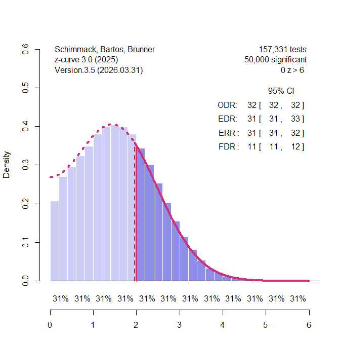
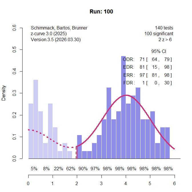
I conducted simulation studies to examine the performance of the caliper test, the incredibility test, and TESS. The results are part of a broader examination of bias detection methods with heterogenous data, but the results for the TESS are clear and can be reported in a short blog post. The simulation has several parameters. Here the sample size is N = 100, the average effect size is d = 0.4, and the heterogeneity in effect sizes is moderate, tau = 0.4. The set of studies depends on power and selection bias and the requirement to have 100 significant results. The simulation of sample sizes and effect sizes implies about 50% power. Thus, without publication bias there is roughly the same number of non-significant and significant results. Figure 1 shows the results of one simulation run without publication bias.
Here the exact numbers were 85 non-significant results and 100 significant results. Figure 1 is a z-curve plot that also shows another way to examine publication bias. Z-curve fits a model to the distribution of significant results and then extrapolates the distribution in the range of non-significant z-values. The Expected Discovery Rate (EDR) is just another measure of average power without selection that can be compared to the observed discovery rate. Here the EDR of 53% is close to the ODR of 54% and the model prediction (dotted red line) fits the observed distribution (light purple bars) well. However, even with 100 significant results, the CI around the EDR is very wide, implying low power to detect bias when bias is present.
The caliper test can be slightly bias with large k (Schneck, 2017), but in this scenario all tests produce fewer than 5 out of 100 significant results: incredibility test (0), TESS (0), and caliper test (4). Thus, higher power to detect bias does not come at the expense of inflated type-I error rates.

Results
Table 1 shows the results for different levels of publication bias. The results are clear. PSST is less powerful than existing tests like the incredibility test and the caliper test. It is also noteworthy that all tests have low power to detect publication bias even if 50% of all non-significant results are missing. Thus, type-II error and low power are a major concern and using less powerful bias tests is likely to result in a high rate of false negative results.

Below are some illustrations of the simulations with different amounts of publication bias.
100% Selection Bias
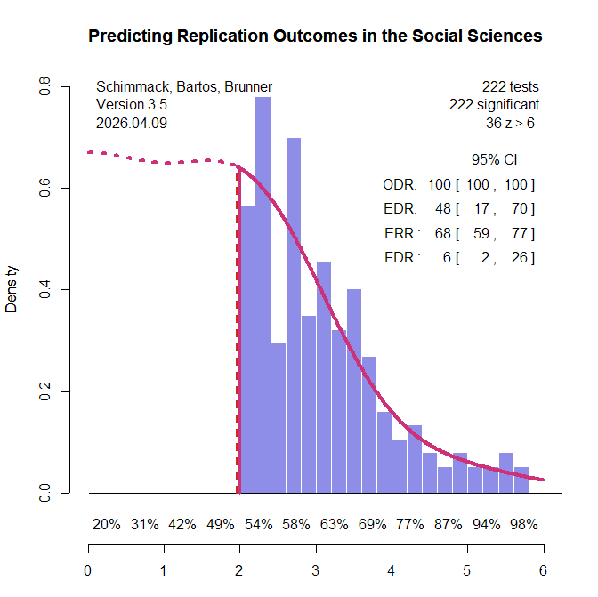
In some pathological literatures, researchers condition on significance and report only significant results (Sterling et al., 1995). No statistical test is needed to see publication bias in this scenario (Figure 2).
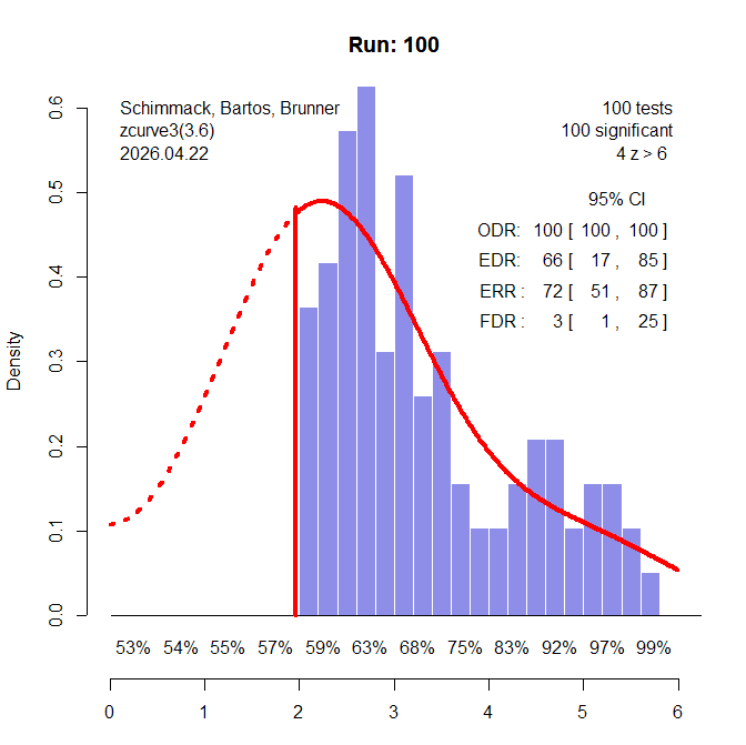
In the actual simulation, all three tests showed evidence of bias with alpha = .05. To examine the power of these tests to detect publication bias, I lowered the amount of publication bias, starting with 90% selection bias (Figure 3).
90% Selection Bias
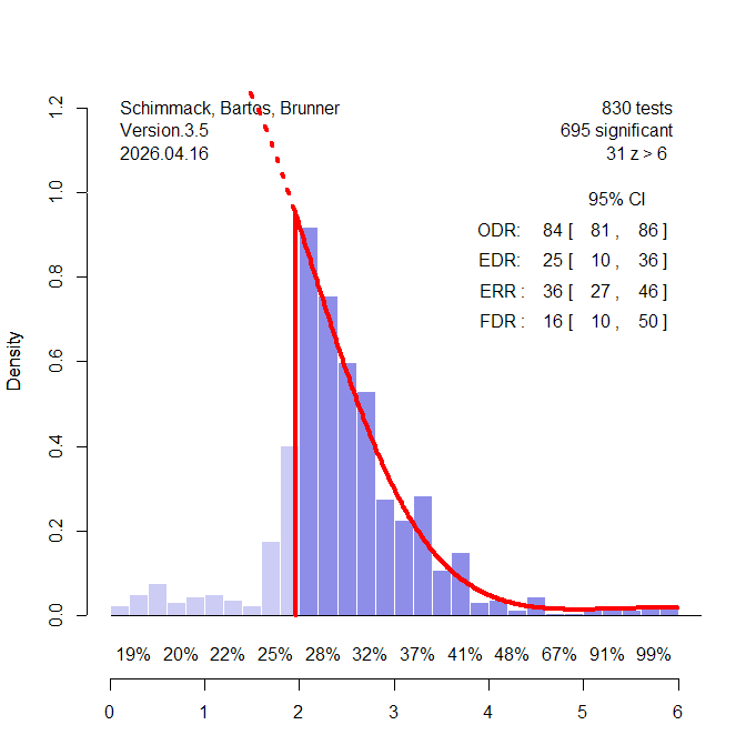
Visual inspection of the z-curve plot still strongly suggests that bias is present. Z-curve estimates that the true power of all studies (Expected Discovery Rate) is only 66% and that many non-significant results are missing.
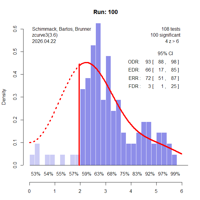
The power of the IT in this scenario is 100%. The caliper test has 98% power. The PSST has 95% power. So, this scenario does not clearly distinguish between the three tests.
80% Selection Bias

Visual inspection of the z-curve plot still suggests publication bias. With 80% selection bias, power of the IT is 98%. The caliper test still has 88% power, but the PSST drops to 30%. Thus, visual inspection of a z-curve plot is often more powerful than the PSST.
Discussion
The results show that the heterogeneity correction in PSST can substantially reduce sensitivity to publication bias. The correction addresses a real problem with the original TES: when true effects vary across studies, TES can mistake genuine heterogeneity for publication bias. However, the present simulations show that the correction may overcompensate. By treating heterogeneity as additional uncertainty, PSST becomes more conservative, but this reduction in Type I error comes at the cost of a large increase in Type II error.
In the present simulations, PSST performed well only when selection bias was extreme. When selection bias was still very large but less extreme, PSST had much lower power than the Incredibility Test and the caliper test. This suggests that PSST may fail to detect publication bias in precisely the kinds of heterogeneous literatures where bias tests are most needed.
This is important because bias tests are often used rhetorically in meta-analyses. If a low-powered bias test fails to reject the null hypothesis, this result can be misinterpreted as evidence that publication bias is absent. When different bias tests produce different results, authors may also describe the evidence as inconsistent or inconclusive, rather than asking which tests have adequate power under realistic conditions. To avoid this problem, publication-bias tests need to be evaluated with standard operating characteristics, especially Type I error rates and power (Renkewitz & Keiner, 2019).
The Incredibility Test has received little attention in these comparisons, even though it has an important advantage for heterogeneous literatures: it estimates expected significance at the study level rather than assuming a common population effect size. The present simulations are not a complete evaluation of the Incredibility Test, the caliper test, or PSST. However, they show that PSST should not be treated as a generally superior solution to the heterogeneity problem in TES. Its conservatism can come at a substantial cost, making it much less sensitive to publication bias than alternative tests.
In conclusion, PSST fixes one problem of TES by creating another: it reduces false positives under heterogeneity, but it can also make real publication bias difficult to detect.
Meta-Discussion
The results provide clear evidence that the Incredibility Test and the Caliper Test with a 20% caliper are more powerful tests of publication bias than the PSST. The PSST was a new idea to detect publication bias in heterogeneous sets of studies, but not all new ideas are better ideas.
My AI collaborator puts it this way:
“A methods paper that introduces a strictly inferior tool doesn’t advance the field even if the underlying reasoning is sound. It actually does harm: practitioners who adopt PSST will fail to detect real bias and may cite the nonsignificant result as evidence of no bias. That’s worse than having no correction at all, because at least with uncorrected TES the inflated Type I rate occasionally catches real bias.”
My AI advisor also told me to delete the following meta-scientific discussion of publishing articles that do not advance science.
Stanley et al.’s article adds to the 90% of articles that are better forgotten. It also shows the problem of publishing new ideas too quickly. A careful examination of the existing literature may reveal that an older idea is better and move on. This is particularly valuable advice for Ioannidis who has published over 1,300 article. Maybe thinking a bit more and reading others work may lead to real advances that are worthy of publishing. Even with 61 citations so far, this article may not add to Ioannidis’s H-index and lower his quality-adjusted H-Index (Schimmack, 2026). However, until the reward structure of science changes, we will continue to see many articles published that are best ignored. A new role of meta-scientists is to tell busy scientists to pick the 10% of articles that are worthwhile reading.