This blog post reports the results of an analysis that predicts variation in scores on the Satisfaction with Life Scale (Diener et al., 1985) from variation in satisfaction with life domains. A bottom-up model predicts that evaluations of important life domains account for a substantial amount of the variance in global life-satisfaction judgments (Andrews & Withey, 1976). However, empirical tests of this prediction fail to show this (Andrews & Withey, 1976).
Here I used the data from the Panel Study of Income Dynamics (PSID) well-being supplement in 2016. The analysis is based on 8,339 respondents. The sample is the largest national representative sample with the SWLS, although only respondents 30 or order are included in the survey.
The survey also included Cantril’s ladder, which was included in the model, to identify method variance that is unique to the SWLS and not shared with other global well-being measures. Andrews & Withey found that about 10% of the variance is unique to a specific well-being scale.
The PSID-WB module included 10 questions about specific life domains: house, city, job, finances, hobby, romantic, family, friends, health, and faith. Out of these 10 domains, faith was not included because it is not clear how atheists answer a question about faith.
The problem with multiple regression is that shared variance among predictor variables contributes to the explained variance in the criterion variable, but the regression weights do not show this influence and the nature of the shared variance remains unclear. A solution to this problem is to model the shared variance among predictor variables with structural equation modeling. I call this method Variance Decomposition Analysis (VDA).
MODEL 1
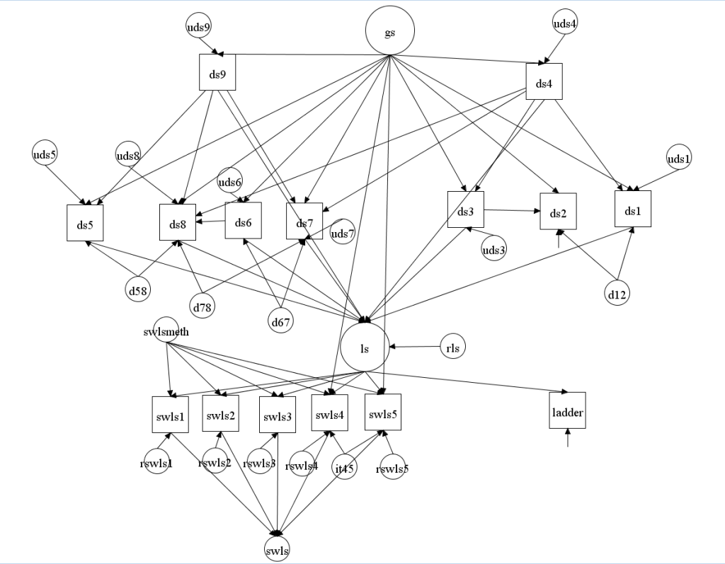
Model 1 used a general satisfaction (GS) factor to model most of the shared variance among the nine domain satisfaction judgments. However, a single factor model did not fit the data, indicating that the structure is more complex. There are several ways to modify the model to achieve acceptable fit. Model 1 is just one of several plausible models. The fit of model 1 was acceptable, CFI = .994, RMSEA = .030.
Model 1 used two types of relationships among domains. For some domain relationships, the model assumes a causal influence of one domain on another domain. For other relationship, it is assumed that judgments about the two domains rely on overlapping information. Rather than simply allowing for correlated residuals, this overlapping variance was modelled as unique factors with constrained loadings for model identification purposes.
Causal Relationships
Financial satisfaction (D4) was assumed to have positive effects on housing (D1) and job (D3). The rational is that income can buy a better house and pay satisfaction is a component of job satisfaction. Financial satisfaction was also assumed to have negative effects on satisfaction with family (D7) and friends (D8). The reason is that higher income often comes at a cost of less time for family and friends (work-life balance/trade-off).
Health (D9) was assumed to have positive effects on hobbies (D5), family (D7), and friends (D8). The rational was that good health is important to enjoy life.
Romantic (D6) was assumed to have a causal influence on friends (D8) because a romantic partner can fulfill many of the needs that a friend can fulfill, but not vice versa.
Finally, the model includes a path from job (D3) to city (D2) because dissatisfaction with a job may be attributed to few opportunities to change jobs.
Domain Overlap
Housing (D1) and city (D2) were assumed to have overlapping domain content. For example, high house prices can lead to less desirable housing and lower the attractiveness of a city.
Romantic (D6) was assumed to share content with family (D7) for respondents who are in romantic relationships.
Friendship (D8) and family (D7) were also assumed to have overlapping content because couples tend to socialize together.
Finally, hobby (D5) and friendship (D8) were assumed to share content because some hobbies are social activities.
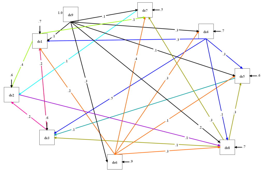
Figure 2 shows the same figure with parameter estimates.
The most important finding is that the loadings on the general satisfaction (GS) factor are all substantial (> .5), indicating that most of the shared variance stems from variance that is shared across all domain satisfaction judgments.
Most of the causal effects in the model are weak, indicating that they make a negligible contribution to the shared variance among domain satisfaction judgments. The strongest shared variances are observed for romantic (D6) and family (D7) (.60 x .47 = .28) and housing (D1) and city (D2) (.44 x .43 = .19).
Model 1 separates the variances of the nine domains into 9 unique variances (the empty circles next to each square) and five variances that represent shared variances among the domains (GS, D12, D67, D78, D58). This makes it possible to examine how much the unique variances and the shared variances contribute to variance in SWLS scores. To examine this question, I created a global well-being measurement model with a single latent factor (LS) and the SWLS items and the Ladder measures as indicators. The LS factor was regressed on the nine domains. The model also included a method factor for the five SWLS items (swlsmeth). The model may look a bit confusing, but the top part is equivalent to the model already discussed. The new part is that all nine domains have a causal error pointing at the LS factor. The unusual part is that all residual variances are named, and that the model includes a latent variable SWLS, which represents the sum score of the five SWLS items. This makes it possible to use the model indirect function to estimate the path from each residual variance to the SWLS sum score. As all of the residual variance are independent, squaring the total path coefficients yields the amount of variance that is explained by a residual and the variances add up to 1.
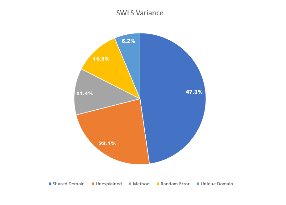
GS has many paths leading to SWLS. Squaring the standardized total path coefficient (b = .67) yields 45% of explained variance. The four shared variances between pairs of domains (d12, d67, d78, d58) yield another 2% of explained variance for a total of 47% explained variance from variance that is shared among domains. The residual variances of the nine domains add up to 9% of explained variance. The residual variance in LS that is not explained by the nine domains accounts for 23% of the total variance in SWLS scores. The SWLS method factor contributes 11% of variance. And the residuals of the 5 SWLS items that represent random measurement error add up to 11% of variance.
These results show that only a small portion of the variance in SWLS scores can be attributed to evaluations of specific life domains. Most of the variance stems from the shared variance among domains and the unexplained variance. Thus, a crucial question is the nature of these variance sources. There are two options. First, unexplained variance could be due to evaluations of specific domains and shared variance among domains may still reflect evaluations of domains. In this case, SWLS scores would have high validity as a global measure of subjective evaluations of domains. The other possibility is that shared variance among domains and unexplained variance reflects systematic measurement error. In this case, SWLS scores would have only 6% valid variance if they are supposed to reflect global evaluations of life domains. The problem is that decades of subjective well-being research have failed to provide an empirical answer to this question.
Model 2: A bottom-up model of shared variance among domains
Model 1 assumed that shared variance among domains is mostly produced by a general factor. However, a general factor alone was not able to explain the pattern of correlations and additional relationships were added to the model Model 2 assume that shared variance among domains is exclusively due to causal relationships among domains. Model fit was good, CFI = .994, RMSEA = .043.
Although the causal network is not completely arbitrary, it is possible to find alternative models. More important, the data do not distinguish between Model 1 and Model 2. Thus, the choice of a causal network or a general factor is arbitrary. The implication is that it is not clear whether 47% of the variance in SWLS scores reflect evaluations of domains or some alternative, top-down, influence.
This does not mean that it is impossible to examine this question. To test these models against each other, it would be necessary to include objective predictors of domain (e.g., income, objective health, frequency of sex, etc.) in the model. The models make different predictions about the relationship of these objective indicators to the various domain satisfactions. In addition, it is possible to include measures of systematic method variance (e.g., halo bias) or predictors of top-down effects (e.g., neuroticism) in the model. Thus, the contribution of domain-specific evaluations to SWLS scores is an empirical question.
Conclusion
It is widely assumed that the SWLS is a valid measure of subjective well-being and that SWLS scores reflect a summary of evaluations of specific life domains. However, regression analyses show that only a small portion of the variance in global well-being judgments is explained by unique variance in domain satisfaction judgments (Andrews & Withey, 1976). In fact, most of the variance stems from the shared variance among domain satisfaction judgments (Model 1). Here I show that it is not clear what this shared variance represents. It could be mostly due to a general factor that reflects internal dispositions (e.g., neuroticism) or method variance (halo bias), but it could also result from relationships among domains in a complex network of interdependence. At present it is unclear how much top-down and bottom-up processes contribute to shared variance among domains. I believe that this is an important research question because it is essential for the validity of global life-satisfaction measures like the SWLS. If respondents are not reflecting about important life domains when they rate their overall well-being, these items are not measuring what they are supposed to measure; that is, they lack construct validity.
With close to 10,000 citations in WebofScience, Ed Diener’s article that introduced the “Satisfaction with Life Scale” (SWLS) is a citation classic in well-being science. While single-item measures are used in large national representative surveys (e.g., General Social Survey, German Socio-Economic Panel, World Value Survey), psychologists prefer multi-item scales because they have higher reliability and therewith also higher validity.
Study 1 in Diener et al. (1985) demonstrated that the SWLS shows convergent validity with single-item measures like Cantril’s ladder, r = .62, .66), and Andrews and Withey’s Delighted-Terrible scale, r = .68, .62. Attesting to the higher reliability of the 5-item SWLS is the finding that the internal consistency was .87 and the retest reliability was r = .82. These results suggest that the SWLS and single-item measures measure a single construct with different amounts of random measurement error.
The important question for well-being scientists who use the SWLS and other global well-being measures is whether these items measure what they are intended to measure. To answer this question, we need to know what life-satisfaction measures are intended to measure.
Diener et al. (1985) draw on Andrews and Withey’s (1976) model of well-being perceptions. Accordingly, life-satisfaction judgments are based on subjective evaluations of important concerns.
Judgments of satisfaction are dependent upon a comparison of one’s circumstances with what is thought to be an appropriate standard. It is important to point out that the judgment of how satisfied people are with their present state of affairs is based on a comparison with a standard which each individual sets for him· or herself; it is not externally imposed. It is a hallmark of the subjective well-being area that it centers on the person’s own judgments, not upon some criterion which is judged to be important by the researcher (Diener, 1984).
This definition of life-satisfaction makes two important points. First, it is assumed that respondents are thinking about their circumstances when they judge their life-satisfaction. That is, we we can think about life-satisfaction as an attitude with an individual’s life as the attitude object. Just like individuals are assumed to think about the important features of Coca Cola when they are asked to report their attitudes towards Coca Cola, respondents are assumed to think about the important features of their lives, when they report their attitudes towards their lives.
The second part of the definition makes it clear that attitudes towards lives are based on subjectively chosen criteria to evaluate lives. Just like individuals may like the taste of Coke or dislike the taste of Coke, the same life circumstance can be evaluated differently by different individuals. Some may be extremely satisfied with an income of $100,000 and some may be extremely dissatisfied with the same income. For students, some students may be happy with a GPA of 2.9, others may be unhappy with the same GPA. The reason is that the evaluation criteria or standards can very across individuals and that there is no objective criterion that is used to evaluate life circumstances. This makes life-satisfaction judgments an indicator of subjective well-being.
The reliance on subjective evaluation criteria also implies that individuals can give different weights to different life domains. For some people, family life may be the most important domain, for others it may be work (Andrews & Withey, 1976). The same point is made by Diener et al. (1985).
For example, although health, energy, and so forth may be desirable, particular individuals may place different values on them. It is for this reason that ,we need to ask the person for their overall evaluation of their life, rather than summing across their satisfaction with specific domains, to obtain a measure of overall life-satisfaction (p. 71).
This point makes sense. If life-satisfaction judgments on evaluations of life circumstances and individuals place different emphasis on different life domains, more important domains should have a stronger influence on global life-satisfaction judgments (Schimmack, Diener, & Oishi, 2002). However, starting with Andrews and Withey (1976), empirical tests of this prediction have failed to confirm it. When individuals are asked to rate the importance of life domains, and these weights are used to compute a weighted average, the weighted average is not a better predictor of global judgments than a simple unweighted average (Rohrer & Schmukle, 2018).
Although this fact has been known since 1974, its theoretical significance has been ignored. There are two possible interpretations of this finding. On the one hand, it could be that importance ratings are invalid. That is, people don’t really know what is important to them and the actual importance is best revealed by the regression weights when global life-satisfaction ratings are regressed on domain satisfaction either across participants or within-participants over time. The alternative explanation is more troubling. In this case, global life-satisfaction judgments are invalid. Maybe these judgments are not based on subjective evaluations of life-circumstances.
Schwarz and Strack (1999) made the point that global life-satisfaction judgments are based on quick heuristics that produce invalid information. The problem of their criticism is that they focused on unstable sources such as mood or temporarily accessible information as the main sources of life-satisfaction judgments. This model fails to explain the high temporal stability of life-satisfaction judgments. (Schimmack & Oishi, 2005).
However, it is possible that stable factors produce systematic method variance in life-satisfaction judgments. For example, Andrews and Withey (1976) suggested that halo bias could influence ratings of domain satisfaction and life-satisfaction. They used informant ratings to rule out this possibility, but their test of this hypothesis was statistically flawed (Schimmack, 2019). Thus, it is possible that a substantial portion of the reliable variance in SWLS scores is halo bias.
Diener et al. (1985) tried to address the problem of systematic measurement error in two ways. First, they included the Marlowe-Crowne Social Desirability (MCSD) scale to measure social desirable responding and found no correlation with SWLS scores, r = .02. The problem is that the MCSD is not a valid measure of socially desriable responding or halo bias, but rather a measure of agreeableness and conscientiousness. Thus, the correlation is better interpreted as evidence that life-satisfaction is fairly independent of these personality traits. Second, Study 3 with 53 elderly residents of Urbana-Champaign included an interview with two trained interviewers. Afterwards, the interviewers made ratings of the interviewees’ well-being. The averaged interviewer’ ratings correlated r = .43 with the self-ratings of well-being. The problem here is that individuals who are motivated to present a positive image in their SWLS ratings are also likely to present a positive image in an interview. Moreover, the conveyed sense of well-being could reflect individuals’ personality more than their life-circumstances. Thus, it is not clear how much of the agreement between self-ratings and interviewer-ratings reflects evaluations of actual life-circumstances.
The most recent review article by Ed Diener was published last year; “Advances and Open Questions in the Science of Subjective Well-Being” (Diener, Lucas, & Oishi, 2018). The article makes it clear that the construct has not changed since 1985.
“Subjective well-being (SWB) reflects an overall evaluation of the quality of a person’s life from her or his own perspective” (p. 1).
“As the term implies, SWB refers to the extent to which a person believes or feels that his or her life is going well. The descriptor “subjective” serves to define and limit the scope of the construct: SWB researchers are interested in evaluations of the quality of a person’s life from that person’s own perspective.” (p. 2)
The authors also explicitly state that subjective well-being measures are subjective because individuals can focus on different aspects of their lives depending on their importance to them.
“it is the subjective nature of the construct that gives it its power. This is due to the fact that different people likely weight different objective circumstances differently depending on their goals, their values, and even their culture” (p. 3).
The fact that global measures allow individuals to assign different weights to different domains is seen as a strength.
Presumably, subjective evaluations of quality of life reflect these idiosyncratic reactions to objective life circumstances in ways that alternative approaches (such as the objective list approach) cannot. Thus, when evaluating the impact of events, interventions, or public-policy decisions on quality of life, subjective evaluations may provide a better mechanism for assessment than alternative, objective approaches (p. 3).
The problem is that this claim requires empirical evidence to show that global life-satisfaction judgments are indeed more valid measures of subjective well-being than simple averages because they properly weigh information in accordance with individuals’ subjective preferences, and since 1976 this evidence has been lacking.
Diener et al.’s (2018) review glosses over this glaring problem for the construct validity of the SWLS and other global well-being measures.
Because most measures are simple self-reports, considerable research addresses the psychometric properties of these types of assessments. This research consistently shows that existing self-report measures exhibit strong psychometric properties including high internal consistency when multiple-item measures are used; moderately strong test-retest reliability, especially over short periods of time; reasonable convergence with alternative measures (especially those that have also been shown to have high levels of reliability and validity); and theoretically meaningful patterns of associations with other constructs and criteria (see Diener et al., 2009, and Diener, Inglehart, & Tay, 2013, for reviews). There is little debate about the quality of SWB measures when evaluated using these traditional criteria.
While it is true that there is little debate, this does not mean that there is strong evidence for the construct validity of the SWLS. The open question is how much respondents are really conducting a memory search for information about important life domains, evaluate these domains based on subjective criteria, and then report an overall summary of these evaluations. If so, subjective importance weights should improve predictions, but they often do not. Moreover, in regression models individual life domains often contribute small amounts of unique variance (Andrews & Withey, 1976), and some important aspects like health often account for close to zero percent of the variance in life-satisfaction judgments.
Convergent Validity
One key feature of construct validity is convergent validity between two independent methods that measure the same construct (Campbell & Fiske, 1959). Ideally, multiple methods are used and it is possible to examine whether the pattern of correlations matches theoretical predictions (Cronbach & Meehl, 1955; Schimmack, 2019). Diener et al. (2018) mention some evidence of convergent validity.
For example, Schneider and Schimmack (2009) conducted a meta-analysis of the correlation between self and informant reports, and they found that there is reasonable agreement (r = .42) between these two methods of assessing SWB.
The problem with this evidence is that the correlation between two measures only shows that both methods are valid, but it is not possible to quantify the amount of valid variance in self-ratings or informant ratings, which requires at least three methods (Andrews & Withey, 1976; Zou, Schimmack, & Gere, 2013). Theoretically, it would be possible that most of the variance in self-ratings is valid and that informant ratings are rather invalid. This is what Andrews and Withey (1976) claimed with estimates of 65% valid variance in self-ratings and 15% valid variance in informant ratings, with a correlation of r = .32. However, their model was incorrect and allowed for method variance in self-ratings to inflate the factor loading of self-ratings.
Zou et al. (2013) avoided this problem by using self-ratings and ratings by two informants as independent methods and found no evidence that self-ratings are more valid than informant ratings; a finding that is mirrored in ratings of personality traits (Anusic et al., 2009). Thus, a correlation of r = .3, implies that 30% of the variance in self-ratings is valid and 30% of the variance in informant ratings is valid.
While this evidence shows that self-ratings of life-satisfaction show convergent validity with informant ratings, it also shows that a substantial portion of the reliable variance in self-ratings is not shared with informants. Moreover, it is not clear what information produces agreement between self-ratings and informant ratings. This question has received surprisingly little attention, although it is critical for the construct validity of life-satisfaction judgments. Two articles have examined this question with opposite conclusions. Schneider and Schimmack (2010) found some evidence that satisfaction in important life domains contributed to self-informant agreement. This finding would support the bottom-up model of well-being judgments that raters are actually considering life circumstances when they make well-being judgments. In contrast, Dobewall, Realo, Allik, Esko, andMetspalu (2013) proposed that personality traits like depression and cheerfulness accounted for self-informant agreement. In this case, informants do not need ot know anything about life circumstances. All they need to know is whether an individual has a positive or negative lens to evaluate their lives. If informants are not using information about life circumstances, they cannot be used to validate self-ratings to show that self-ratings are based on evaluations of life circumstances.
Diener et al. (2018) cite a number of additional findings as evidence of convergent validity.
Physiological measures, including brain activity (Davidson, 2004) and hormones (Buchanan, al’Absi, & Lovallo, 1999), along with behavioral measures such as the amount of smiling (e.g., Oettingen & Seligman, 1990; Seder & Oishi, 2012) and patterns of online behaviors (Schwartz, Eichstaedt, Kern, Dziurzynski, Agrawal et al., 2013) have also been used to assess SWB. (p. 7).
This evidence has several limitations. First, hormones do not reflect evaluations and are at best indirectly related to life-evaluations. Asymmetries in prefrontal brain activity (Davidson, 2004) have been shown to reflect approach and avoidance motivation more than pleasure and displeasure, and brain activity is a better measure of momentary states than the evaluation of fairly stable life circumstances. Finally, they also may reflect individuals’ personality more than their life circumstances. The same is true for the behavioral measures. Most important, correlations with a single indicators do not provide information about the amount of valid variance in life-satisfaction judgments. To quantify validity it is necessary to examine these findings within a causal network (Schimmack, 2019).
Diener et al. (2019) agree with my assessment in their final conclusions about measurement of subjective well-being.
The first (and perhaps least controversial) is that many open questions remain regarding the associations among different SWB measures and the extent to which these measures map on to theoretical expectations; therefore, understanding how the measures relate and how they diverge will continue to be one of the most important goals of research in the area of SWB. Although different camps have emerged that advocate for one set of measures over others, we believe that such advocacy is premature. More research is needed about the strengths, weaknesses, and relative merits of the various approaches to measurement that we have documented in this review (p. 7).
The problem is that well-being scientists have made no progress on this front since Andrews and Withey (1976) conducted the first thorough construct validation studies. The reason is that social and personality psychology suffers from a validation crisis (Schimmack, 2019). Researchers simply assume that measures are valid rather than testing it or they use necessary, but insufficient criteria like internal consistency (alpha), retest reliability as evidence. Moreover, there is a tendency to ignore inconvenient findings. As a result, 40 years after Andrews and Withey’s (1976) seminal article was published, it remains unclear (a) whether respondents aggregate information about important life domains to make global judgments, (b) how much of the variance in life-satisfaction judgments is valid, and (c) which factors produce systematic biases in life-satisfaction judgments that may lead to false conclusions about the causes of life-satisfaction and to false policy recommendations.
Health is probably the best example to illustrate the importance of valid measurement of subjective well-being. It makes intuitive sense that health has an influence on well-being. Illness often disables individuals from pursuing their goals and enjoying life as everybody who had the flu knows. Diener et al. (2018) agree.
“One life circumstance that might play a prominent role in subjective well-being is a person’s health” (p. 15).
It is also difficult to see how there could be dramatic individual differences in the criteria that are used to evaluate health. Sure, fitness levels may be a matter of personal preference, but nobody is enjoying a stroke, heart attack, or cancer, or even having the flu.
Thus, it was a surprising finding that health seemed to have a small influence on global well-being judgments.
“Initial research on the topic of health conditions often concluded that health played only a minor role in wellbeing judgments (Diener et al., 1999; Okun, Stock, Haring, & Witter, 1984).”
More problematic was the finding that subjective evaluations of health seemed to play no role in these judgments in multivariate analyses that controlled for shared variance among ratings of several life domains. For example, in Andrews and Withey’s (1976) studies satisfaction with health contributed only 1% unique variance in the global measure.
In contrast, direct importance ratings show that health is rated as the second most important domain (Rohrer & Schmukle, 2018).
Thus, we have to conclude that health doesn’t seem to matter for people’s subjective well-being. Or we can conclude that global measures are (partially) invalid measures because respondents do not weigh life domains in accordance with their importance. This question clearly has policy relevance as health care costs are a large part of wealthy nations’ GDP and financing health care is a controversial political issue, especially in the United States. Why would this be the case, if health is actually not important for well-being. We could argue that it is important for life expectancy (Veenhoven’s happy life-years) or that it matters for objective well-being, but not for subjective well-being, but clearly the question why health satisfaction plays a small role in global measures of subjective well-being is an important one. The problem is that 40 years of well-being science have passed without addressing this important question. But as they say, better late than never. So, let’s get on with it and figure out how responses to global well-being questions are made and whether these cognitive processes are in line with the theoretical model of subjective well-being.
In 1976, Andrews and Withey published a groundbreaking book on the measurement of well-being. Although their book has been cited over 2,000 times, including influential articles like Diener’s 1984 and 1999 Psychological Bulletin articles on Subjective Well-Being, it is likely that many people are not familiar with the book because books are not as accessible as online articles. The aim of this blog post is to review and comment on the main points made by Andrews and Withey.
CHAPTER 1: Introduction
A&W (wink) believed that well-being indicators are useful because they reflect major societal forces that influence individuals’ well-being.
“In these days of growing interdependence and social complexity we need more adequate cues and indicators of the nature, meaning, pace, and course of social change” (p. 1).
Presumably, A&W would be pleasantly surprised about the widespread use of well-being surveys for this purpose. Well-being questions are included in the General Social Survey, The German Socio-Economic Panel Study, the World Value Survey, and Gallup’s World Poll and the daily survey of Americans’ well-being and health.
A&W saw themselves as part of a broader movement towards evidence based public policy.
The social indicator “movement” is gaining adherents all over the world. … Several facets of these definitions reflect the basic perspectives of the social indicator effort. The quest is for a limited yet comprehensive set of coherent and significant indicators, which can be monitored over time, and which can be disaggregated to the level of the relevant social unit (p. 4).
Objective and Subjective Indicators
A&W criticize the common distinction between objective and subjective indicators of well-being. Objective indicators such as hunger, pollution, or unemployment are factors that are universally considered bad for individuals are typically called objective indicators.
A&W propose to distinguish three features of indicators.
Thus, it may be more helpful and meaningful to consider the individualistic or consensual aspects of phenomena, the private or public accessibility of evidence, and the different forms and patterns of behavior needed to change something rather than to cling to the more simplistic notions of objective and subjective.
They propose to use “perceptions of well-being” as a social indicator. This indicator is individualistic, private, and may require personalized interventions to change them.
The work of engineers, industrialists, construction workers, technological innovators, foresters, and farmers who alter the physical and biological environment is matched by educators, therapists, advertisers, lovers, friends, ministers, politicians, and issue advocates who are all interested and active in constructing, tearing down, and remodeling subjective appreciations and experiences. (p. 6)
A&W argue that measuring “perceptions of well-being” is important because citizens of modern societies share the belief that societies should maximize well-being.
The promotion of individual well-being is a central goal of virtually all modern societies, and of many units within them. While there are real and important differences of opinion-both within societies and between them-about how individual well-being is to be maximized, there is nearly universal agreement that the goal itself is a worthy one and is to be actively pursued. (p. 7).
Research Goals
A&W’s goal was to develop a set of indicators (not just one) that fulfill several criteria that can be considered validation criteria.
1. Content validity. Their coverage should be sufficiently broad to include all the most important concerns of the population whose well-being is to be monitored. If the relevant population includes demographic or cultural subgroups that might be the targets of separate social policies, or that might be affected differentially by social policies, the indicators should have relevance for each of the subgroups as well as for the whole population.
2. Construct Validity. The validity (i.e., accuracy) with which the indicators are measured should be high, and known.
3. Parsimony and Efficiency: It should be possible to measure the indicators with a high degree of statistical and economic efficiency so that it is feasible to monitor them on a regular basis at reasonable cost.
4. Flexibility: The instrument used to measure the indicators should be flexible so that it can accommodate different trade-offs between resource input, accuracy of output, and degree of detail or specificity.
In short, the indicators should be measured with breadth, relevance, efficiency, validity, and flexibility. (p. 8).
A&W then list several specific research questions that they aimed to answer.
1. What are the more significant general concerns of the American people?
2. Which of these concerns are relevant to Americans’ sense of general wellbeing?
3. What is the relative potency of each concern vis-a.-vis well-being?
4. How do the relevant concerns relate to one another?
5. How do Americans arrive at their general sense of well-being?
6. To what extent can Americans easily identify and report their feelings about well-being?
7. To what extent will they bias their answers?
8. How stable are Americans’ evaluations of particular concerns?
9. How comparable are various subgroups within the American population with respect to each of the questions above?
Although some of these questions have been examined in great detail others have been neglected in the following decades of well-being research. In particular, very little attention has been paid to questions about the potency (strength of influence) of different concerns for global perceptions of well-being, and to the question how different concerns are related to each other. In contrast, the stability of well-being perceptions has been examined in numerous longitudinal studies (see Anusic & Schimmack, 2016, for the most recent meta-analysis).
Usefulness
A&W “propose six products of value to social scientists, to policymakers and implementers of policy, and to people who want to influence the course of society” (p. 9).
1. Repeated measurement of well-being perceptions can be used to see whether (humans’) lives are betting better or worse.
2. Comparison of groups (e.g., men vs. women, White vs. Black Americans) can be used to examine equity and inequity in well-being.
3. Positive or negative correlations among domains can be informative. For example, marital satisfaction may be positively or negatively correlated to each other, and this evidence has been used to study work-family or work-live balance.
4. It is possible to see how much well-being perceptions are based on more objective aspects of life (job, housing) versus more abstract aspects such as values or meaning.
5. It is informative to see what domains have a stronger influence on well-being perceptions, which shows people’s values and priorities.
6. It is important to know whether people appreciate actual improvement. For example, a drop in crime rates is more desirable if citizens also feel safer. “The appreciation of life’s conditions would often seem to be as important as what those conditions actually are” (p. 10).
One may justifiably claim, then, that people’s evaluations are terribly important: to those who would like to raise satisfactions by trying to meet people’s needs, to those who would like to raise dissatisfactions and stimulate new challenges, to those who would suppress or reduce feelings and public expressions of discontent, and above all, to the individuals themselves. It is their perceptions of their own well-being, or lack of well-being, that ultimately define the quality of their lives (p. 10).
BASIC CONCEPTS AND A CONCEPTUAL MODEL
The most important contribution of A&W is their conception of well-being as a broad evaluations of important life domains. We might think about a life as a pizza with several slices that have different toppings. Some are appealing (say ham and pineapple) and some are less appealing (say sardines and olives). Well-being is conceptualized as the sum or average of evaluations of the different slices. This view of well-being is now called the bottom-up model after Diener (1984).
We conceive of well-being indicators as occurring at several levels of specificity. The most global indicators are those that refer to life as a whole; they are not specific to anyone particular aspect of life (p. 11).
Mostly forgotten is A&W’s distinction between life domains and criteria.
Domains and Criteria
Domains are essentially different slices of the pizza of life such as work, family, health, recreation.
Criteria are values, standards, aspirations, goals, and-in general-ways of judging what the domains of life afford. In modern research, they are best represented by models of human values or motives, such as Schwartz’s model of human values. Thus, life domains or aspects can be desirable or undesirable because the foster or block fulfillment of universal needs for safety, freedom, pleasure, connectedness, and achievement to name a few.
The quality of life is not just a matter of the conditions of one’s physical, interpersonal and social setting but also a matter of how these are judged and evaluated by oneself and others. The values that one brings to bear on life are in themselves determinants of one’s assessed quality of life. Leave the situations of life stable and simply alter the standards of judgment and one’s assessed quality of life could go up or down according to the value framework. (p. 13).
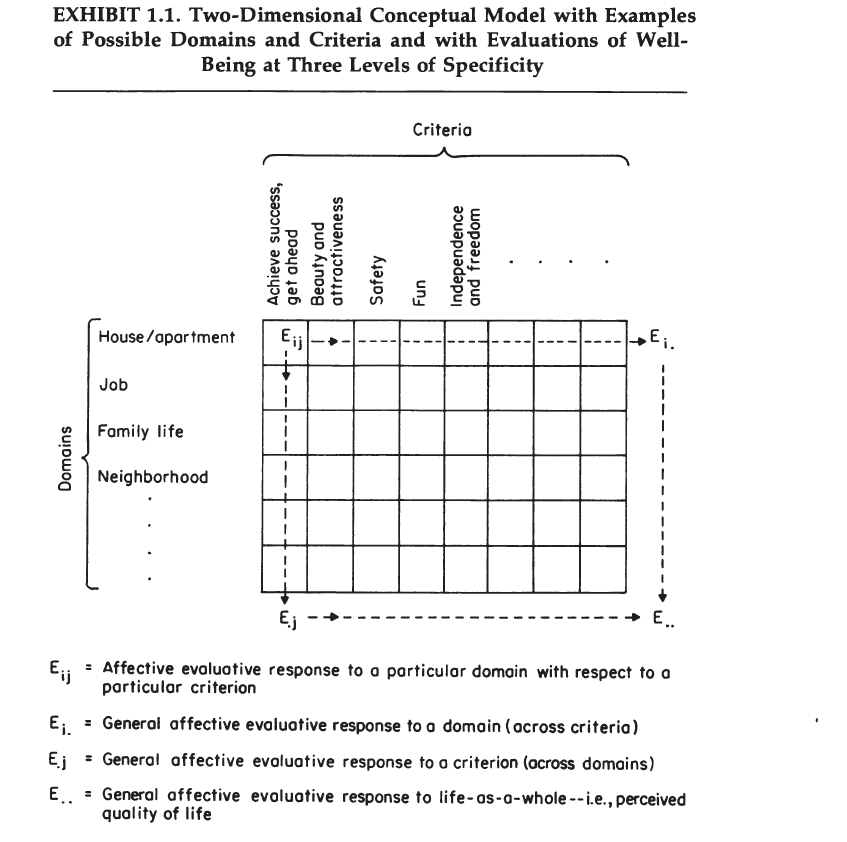
A Conceptual Model
A&W’s Exhibit 1.1 shows a grid of life domains and evaluation criteria (values). According to their bottom-up model, perceptions of well-being are an integrated summary of these lower-order evaluations of specific life domains.
“The diagram is also intended to imply that global evaluations-i.e., how a person feels about life as a whole-may be the result of combining the domain evaluations or the criterion evaluations” (p. 14)
METHODS AND DATA
The Measurement of Affective Evaluations
A&W proposed that perceptions of well-being are based on two modes of evaluation.
The basic entries in the model, just described, are what we designate as “affective evaluations.” The phrase suggests our hypothesis that a person’s assessment of life quality involves both a cognitive evaluation and some degree of positive and/or negative feeling, i.e., “affect.”
One mode is cognitive and could be performed by a computer. Once objective circumstances are known and there are clear criteria for evaluation, it is possible to compute the discrepancy. For example, if a person needs $40,000 a year to afford housing, food, and basic necessities, an income of $20,000 is clearly inadequate, whereas an income of $70,000 is more than adequate. However, A&W also propose that evaluations have a feeling or affective component. That is, the individual who earns only $20,000 may feel worse about their income, while the individual with a $70,000 income may feel good about their income.
Not much progress has been made in terms of distinguishing affective or cognitive evaluations, especially when it comes to evaluations of specific life domains. One problem is that it is difficult to measure affective reactions and that self-reports of feelings may simply be cognitive judgments. It is therefore easier to think about well-being “perceptions” as evaluations, without trying to distinguish between cognitive and affective evaluations.
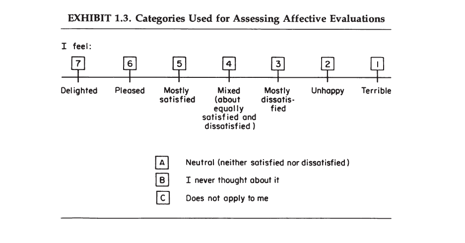
Both global and more specific evaluations are measured with rating scales. A&W favored the delighted-terrible scale, but it didn’t catch on. Much more commonly used is Cantril’s Ladder or life-satisfaction or happiness questions.
In the next section of this interview/questionnaire we want to find out how you feel about various parts of your life, and life in this country as you see it. Please tell me the feelings you have now-taking into account what has happened in the last year and what you expect in the near future.
A&W were concerned that a large proportion of respondents’ report high levels of satisfaction because they are merely satisfied, but not really happy or delighted. They also wanted a 7-point scale and suggested that more categories would not produce more sensitive responses, while a 7-point scale is clearly preferable to the 3-point happiness measure that is still used in the General Social Survey. They also wanted a scale where each response option is clearly labelled, while some scales like Cantril’s ladder only label the most extreme options (best possible life, worst possible life).
Data Sources
A&W conducted several cross-sectional surveys.
CHAPTER 2: Identifying and Mapping Concerns
Research Strategy
The basic strategy of our approach was first to assemble a very large number of possible life concerns and to write questionnaire items to tap people’s feelings, if any, about them. Then, having administered these items to broad samples of Americans, we used the resulting data to empirically explore how people’s feelings about these items are organized.
IDENTIFYING CONCERNS
The task of identifying concerns involved examining four different types of sources.
One source was previous surveys that had included open questions about people’s concerns. Two examples of such items are:
All of us want certain things out of life. When you think about what really matters in your own life, what are your wishes and hopes for the future? In other words, if you imagine your future in the best possible light, what would your life look like then, if you are to be happy? (Cantril, 1965)
In this study we are interested in people’s views about many different things. What things going on in the United States these days worry or concern you? (Blumenthal et aI., 1972)
In our search for expression of life concerns, we examined data from these very general unstructured questions in eight different surveys.
A second type of source was structured interviews, typically lasting an hour or two with about a dozen people of heterogeneous background.
A third type of source, particularly useful for expanding our list of criterion-type concerns, was previously published lists of values.
This information was used to create items that were administered in some of the surveys.
MAPPING THE CONCERNS
Given the list of 123 concern items, the next step was to explore how they fit together in people’s thinking.
Maps and the Mapping Process
Selecting and Clustering Concern-Level Measures
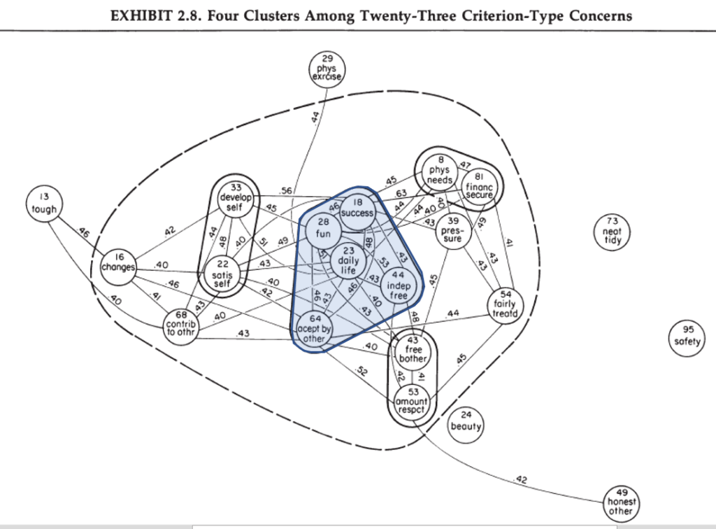
A&W’s work identified clusters of concerns that are often included in surveys of domain satisfaction such as work (green), recreation (orange), standard of living (purple), housing (light blue), health (red), and family (dark blue).
The map for criteria, shows that the most central values are hedonism (having fun), achievement, acceptance and affiliation (accept by other) and freedom.
These findings are consistent with modern conceptions of well-being as the freedom to seek pleasure and to avoid pain (Bentham).
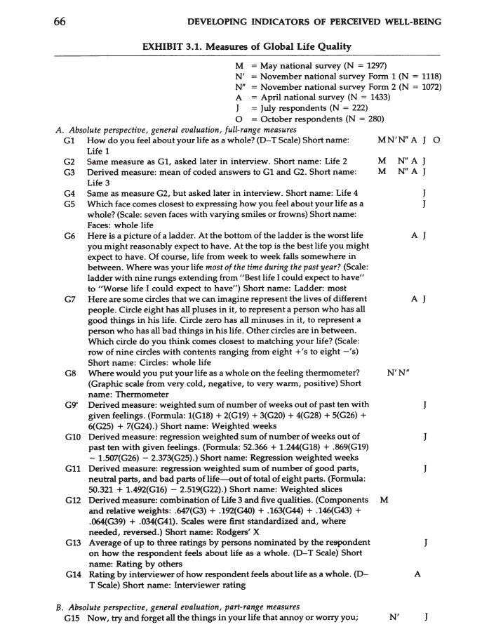
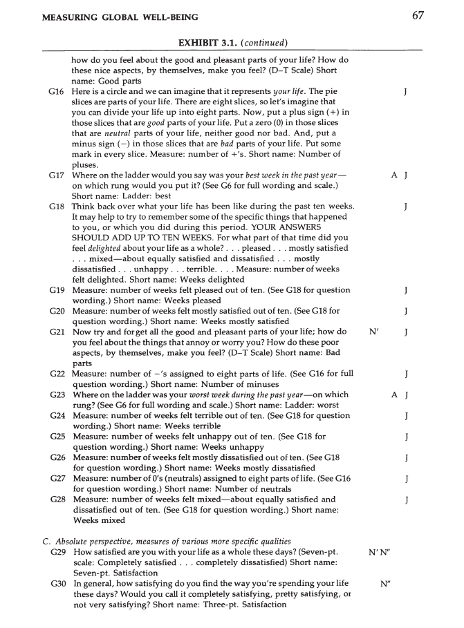
CHAPTER 3: Measuring Global Well-Being
A&W compiled 68 items that had been used to measure global well-being.
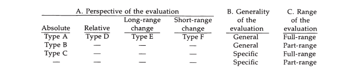
Formal Structure of the Typology
A&W provided a taxonomy of the various global measures.
Accordingly, measures can differ in the perspective of the evaluation, the generality of the evaluation, and the range of the evaluation. For the measurement of global well-being general measures that cover the full-range from an absolute perspective are most widely used.
“We find that the Type A measures, involving a general evaluation of the respondent’s life-as-a-whole from an absolute perspective, tend to cluster together into what we shall call the core cluster” (p. 76).
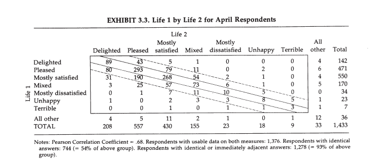
A study of the retest stability for the same item in the same survey showed a retest correlation of r = .68. This estimate for the reliability of a single global well-being rating has been replicated in numerous studies (see Ansic & Schimmack, 2005; Schimmack & Oishi, 2005; for meta-analyses).
A&W also provided some evidence about measurement invariance across subgroups (gender, racial groups, age groups) and found very similar results.
“The results (not shown) indicated very substantial stabilities across the subgroups. In nearly all cases the correlations within the subgroups were within 0.1 of the correlations within the total population.” (p. 83).
The next results show that different global well-being measures tend to be highly correlated with each other. Exceptions are the 3-point happiness scale in the GSS, which lacks sensitivity, and the affect measure because affect measures show some discriminant validity from life evaluations (Zou, Schimmack, & Gere, 2013). That is, an individuals’ perception of well-being is not fully determined by their perception of how much pleasure versus displeasure they experienced.
A principal component analysis showed items with high loadings that best capture the shared variance among global well-being measures.
The results show that the 7-point delighted-terrible (Life 1, Life 2) or a 7-point happiness scale capture this variance well.
These results lead A&W to conclude that these measures are valid and useful indicators of well-being.
“We believe the Type A measures clearly deserve our primary attention. Thus, it is reassuring to find that the Type A measures provide a statistically defensible set of general evaluations of the level of current wellbeing” (p. 106).
CHAPTER 4: Predicting Global Well-Being: I
A&W argue that statistical predictors of global well-being ratings provide useful information about the cognitive processes (what is going on in the minds of respondents) underlying well-being ratings.
Finding a statistical model that fits the data has real substantive interest, as well as methodological, because in these data the statistical model can also be considered as a psychological model. Not only is the model that method of combining feelings that provides the best predictions, it is also our best indication of what may go on in the minds of the respondents when they themselves combine feelings about specific life concerns to arrive at global evaluations. Thus, our statistical model can also be considered as a simulation of psychological processes (p. 109).
This assumption is reasonable as ratings are clearly influenced by some information in memory that is activated during the formation of a response. However, the actual causal mechanism can be more complicated. For example, job satisfaction may be correlated with global well-being only because respondents’ think about income and income satisfaction is related with job satisfaction. Moreover, Diener (1984) pointed out that causality may flow from global well-being to domain satisfaction, which is now called a top-down process. Thus, rather than job satisfaction being used to make a global well-being judgment, respondents’ affective disposition may influence their job satisfaction.
A&W’s next finding has been replicated and emphasized in many review articles on well-being.
The prediction of global well-being from the demographic characteristics of the respondents produced straightforward results that have proved surprising to some observers: The demographic variables, either singly or jointly, account for very little of the variance in perceptions of global well-being (less than 10 percent), and they add nothing to what can be predicted (more accurately) from the concern measures (p. 109).
This finding has also been misinterpreted as evidence that objective life circumstances have a small influence on well-being. The problem with this interpretation is that demographic variables do not represent all environmental influences and many of them are not even environmental factors (e.g., sex, age, race). It is true, however, that there are relatively small differences in well-being perceptions across different groups. The main exception is a persistent gap in well-being of White and Black Americans (Iceland & Ludwig-Dehm, 2019).
A&W conducted numerous tests to look for non-linear relationships. For example, only very low income satisfaction or health satisfaction may be related to global well-being if moderate levels of income or health are sufficient to be satisfied with life. However, they found no notable non-linear relationships.
However, after examining many associations between feelings about specific life concerns and life-as-a-whole, we conclude that substantial curvilinearities do not occur when affective evaluations are assessed using the DelightedTerrible Scale (p. 110).
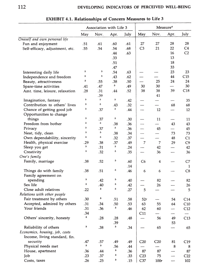
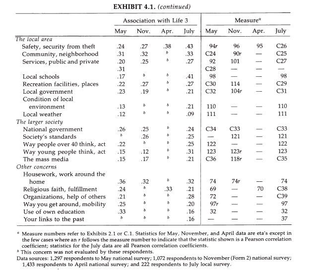
Exhibit 4.1 shows simple linear correlations of various life concerns with the averaged repeated ratings on the Delighted-Terrible scale (Life 3).
The main finding is that all correlations are positive, most are moderate, and some are substantial (r > .5), such as the correlations for fun/enjoyment, self-efficacy, income, and family/marriage.
It is important to interpret differences in the strength of correlations with caution because several factors influence how strong these correlations are. One factor is the amount of variability in a predictor variable. For example, while incomes can vary dramatically, the national government is the same for everybody. Thus, there is no variability in government that can produce variability in well-being across respondents; although perceptions of government can vary and could influence well-being perceptions. Keeping this caveat in mind, the results suggest that concerns about standard of living and family life seem to matter most. Interestingly, health is not a major factor, but once again, this might simply reflect relatively small variability in actual health, while health may become more of a concern later in life.
Nevertheless, while the causal processes that produce these correlations are unclear, any theory of well-being has to account for this robust pattern of correlations. between global well-being perceptions and concerns.
MULTIVARIATE PREDICTION OF LIFE 3
Regression analysis aims to identify variables that make a unique contribution to the prediction of an outcome. That is, they share variance with the outcome that is not shared by other predictor variables.
As mentioned before, there was no evidence of marked non-linearity, so all variables were entered as measured without transformation or quadratic terms. A&W also examined potential interaction effects, but did not find evidence for these either.
Weighting Schemes
One of the most important analyses was the exploration of different weighting schemes. Intuitively, it makes sense that some domains are more important than others (e.g., standard of living vs. weather). If this is the case, a predictor that weights standard of living more should be a better predictor of well-being than a predictor that weights all concerns equally.
A&W found that a simple average of 12 concerns was highly correlated with the global measure.
Several explorations provide consistent and clear answers to these questions. A simple summing of answers to any of certain alternative sets of concern items (coded from 1 to 7 on the Delighted-Terrible Scale) provides a prediction of feelings about life-as-a-whole that correlates rather well with the respondent’s actual scores on Life 3. Using twelve selected concerns12 (mainly domains) and data from the May respondents, this correlation was .67 (based on 1,278 cases); using eight selected concerns13 (all criteria) and data from the April respondents, the correlation was .77 (based on 1,070 cases). These relatively high values obtain in subgroups of the population as well as in the population as a whole: When the sum of answers to eight of the April concern items was correlated with Life 3 in twenty-one different subgroups of the national adult population, the correlation was never lower than .70 nor higher than .82. (p. 118).
However, more important is the question whether other weighing schemes produce higher correlations, and the important finding is that optimal weights (using regression coefficients) produced only a small improvement in the multiple correlation.
What is extremely interesting is that the optimally weighted combination of concern measures provides a prediction of Life 3 that is, at most, only modestly better than that provided by the simple sum. In the May data, the previous correlation of .67 could be increased to .71 by optimally weighting the twelve concern measures.
A&W conclude that a model with equal weights is a parsimonious and good model of well-being.
Our conclusion is that the introduction of weights when summing answers to the concern measures is likely to produce a modest improvement, but that even a simple sum of the answers provides a prediction that is remarkably close to the best that can be statistically derived.
However, the use of a fixed regression weight implies that all respondents attach the same importance of different domains. It is plausible that this is not the case. For example, some people live to work and others work to live. So, work would have different importance for different respondents. A&W tested this by asking respondents about the importance of several domains and used this information to weight concerns on a person by person basis. They found that this did not improve prediction.
The significant finding that emerged is that there was no possible use of these importance data that produced the slightest increase in the accuracy with which feelings about life-as-a-whole could be predicted over what could be achieved using an optimally weighted combination of answers to the concern measures alone.Although a number of questions remain with respect to the nature and meaning of the importance measures (some are explored in chap. 7), we have an unambiguous answer to our original question: Data about the importance people assign to concerns did not increase the accuracy with which feelings about life-as-a-whole could be predicted (p. 119).
This surprising result has been replicated numerous times (Rohrer & Schmukle, 2018). However, nobody has attempted to explain why importance weights do not improve prediction. After all, it is theoretically nonsensical within A&W’s theoretical framework to say that work, family, and health are very important, to be extremely dissatisfied in these domains, and then to report high global well-being. If global well-being judgments are, indeed, based on information about concerns and life domains, then important life domains should have a stronger relationship with global well-being ratings than unimportant domains (cf. Schimmack, Diener, & Oishi, 2002).
While I share A&W’s surprise, I am much less pleased by this finding.
Our results point to a simple linear additive one, in which an optimal set of weights is only modestly better than no weights (i.e. equal weights).19 We confess to both surprise and pleasure at these conclusions (p. 120).
A&W are pleased because a simple additive, linear model is simple and science favors simple models, when they fit actual data reasonably well, which seems to be the case here.
However, A&W are too quick to interpret their results as support for their bottom-up model of well-being, where everybody weights concerns equally and well-being perceptions depend only on the relative standing in life domains (good job, happy marriage, etc.).
Interpreted in this light, the linear additive model suggests that somehow individuals themselves “add up” their joys and sorrows about specific concerns to arrive at a feeling about general well-being. It appears that joys in one area of life may be able to compensate for sorrows in other areas; that multiple joys accumulate to raise the level of felt well-being; and that multiple sorrows also accumulate to lower it.
In discussing these findings with various colleagues and commentators, the question has sometimes been raised as to whether the model implies a policy of “give them bread and circuses.” The model does suggest that bread and circuses are likely to increase a population’s sense of general well-being. However, the model does not suggest that bread and circuses alone will ensure a high level of well-being. On the contrary, it is quite specific in noting that concerns that are evaluated more negatively than average (e.g., poor housing, poor government, poor health facilities, etc.) would be expected to pull down the general sense of well-being, and that multiple negative feelings about life would be expected to have a cumulative impact on general well-being.
At least at this stage of the investigation in Chapter 4 other, more troubling interpretations of the results are possible. Maybe most of the variance in these evaluative judgments are response biases and social desirable responding. This alone could produce strong correlations and they would be independent of the actual concerns that are being rated. Respondents could rate the weather on Mars and we would still see that those who are more satisfied with the weather on Mars have higher global well-being.
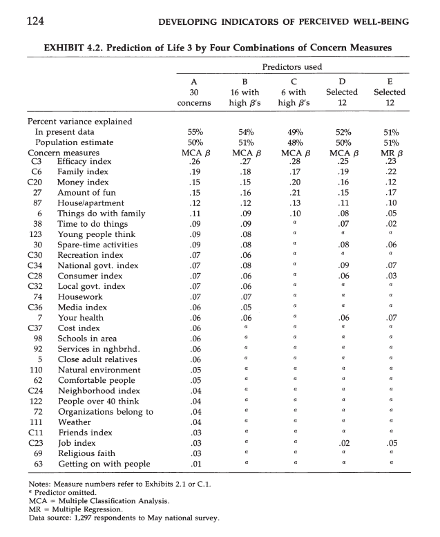
However, A&W’s subsequent analyses are inconsistent with their conclusions. Exhibit 4.2 shows the regression weights for various concerns that are sorted by the amount of unique contribution to the global impressions. It is clear that averaging the top 12 concerns would give a measure that is more strongly related to global well-being than averaging the last 12 concerns. Thus, domains do differ in importance. The results in the last column (E) are interesting because here 12 domains explain 51% of the total variance, but squaring the regression coefficients provides only 17% of variance, which implies that most of the explained variance stems from variance that is shared among the predictor variables. Thus, it is important to examine the nature of this shared variance more closely. In this mode, the first five domains account for 15 of the 17 percent in total. These domains are efficacy, family, money, fun, and housing. Thus, there is some support for the bottom-up model for some domains, but most of the explained variance may stem from shared method variance between concern ratings and well-being ratings.
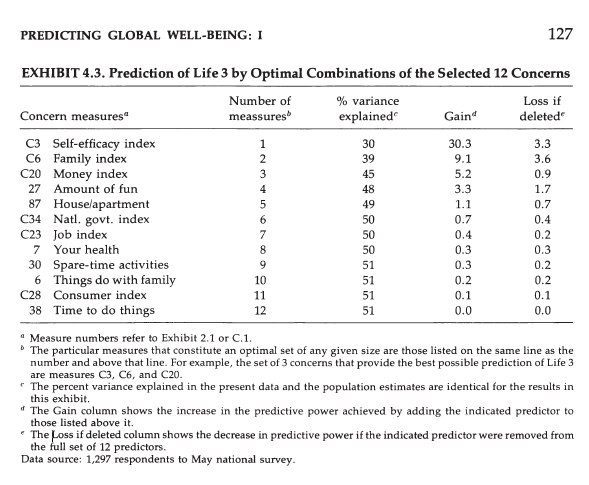
Exhibit 4.3 confirms this with a stepwise regression analysis where concerns are entered according to their unique importance. Self-efficacy alone accounts for 30% of the explained variance. Then family adds 9%, money adds 5%, fun adds 3%, and housing 1%. The remaining variables add less than 1% individually.
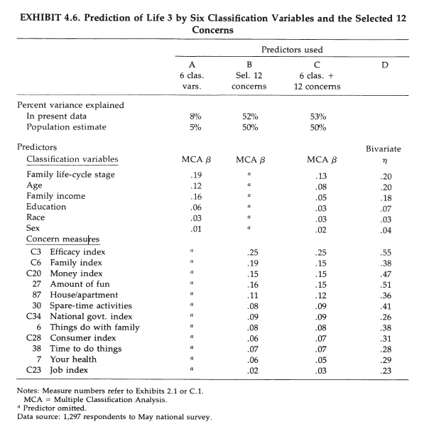
Exhibit 4.4 shows that demongraphic variables are weak predictors of well-being ratings and that these relationships are weakened when concerns are added as predictors (column 3).
This suggests that effects of demongraphic variables are at least partially mediated by concerns (Schimmack, 2008). For example, the influence of income on well-being ratings could be explained by the effect of income on satisfaction with money, which is a unique predictor of well-being ratings (income -> money satisfaction-> life satisfaction). The limitation of regression analysis is that it does not show which of the concerns mediates the influence of income. A better way to examine mediation is to test mediation models with structural equation modeling (Baron & Kenny, 1986).
A&W draw the conclusion that there are no major differences in perceived well-being between social groups. As mentioned before, this is only partially correct. The GSS shows consistent racial differences in well-being.
“The conclusion seems inescapable that there is no strong and direct relationship between membership in these social subgroups and feelings about life-as-a-whole” (p. 142).
CHAPTER 5: Predicting Global Well-Being: II
Chapter 5 does not make a major novel contribution. It mainly explores how concerns are related to the broader set of global measures. The results show that the findings in Chapter 4 generalize to other global measures.
CHAPTER 6: Evaluating the Measures of Well-Being
Chapter 6 tackles the important question of construct validity. Do global measures measure individuals’ true evaluations of their lives?
How good are the measures of perceived well-being reported in previous chapters of this book? More specifically, to what extent do the data produced by the various measurement methods indicate a person’s true feelings about his life? (p. 175).
A&W note several reasons why global ratings may have low validity.
Unfortunately, evaluating measures of perceived well-being presents formidable problems. Feelings about one’s life are internal, subjective matters. While very real and important to the person concerned, these feelings are not necessarily manifested in any direct way. If people are asked about these feelings, most can and will speak about them, but a few may lie outright, others may shade their answers to some degree, and probably most are influenced to some extent by the framework in which the questions are put and the format in which the answers are expected. Thus, there is no assurance that the answers people give fully represent their true feelings. (p. 176)
ESTIMATION OF THE VALIDITY AND ERROR COMPONENTS OF THE MEASURES
Measurement Theory and Models
A&W are explicit in their ambition. They want to estimate the proportion of variance in global well-being measures that reflects respondents’ true evaluations of their lives. They want to separate this variance from random measurement error, which is relatively easy, and systematic measurement error, which is hard (Campbell & Fiske, 1959).
The analyses to be reported in this major section of the chapter begin from the fact that the variance of any measure can be partitioned into three parts: a valid component, a correlated (i.e., systematic) error component, and a random error (or “residual”) component. Our general analysis goal is to estimate, for measures of different types, from different surveys, and derived from different methods, how the total variance can be divided among these three components (p. 178).
A “validity coefficient,” as this term is commonly used by social scientists, is the correlation (Pearson’s product-moment r) between the true conditions and the obtained measure of those conditions. The square of the validity coefficient gives the proportion of observed variance that is true variance; e.g., a measure that has a validity coefficient of .8 contains 64 percent valid variance; similarly, a measure that contains 49 percent valid variance has a validity of .7. (p. 179; cf. Schimmack, 2010).
One source of systematic measurement error are response sets such as aquiescence bias. Another one is halo bias.
A special form of bias is what is sometimes known as “halo.” One would hope that a respondent, when answering a series of questions about different aspects of something-e.g., his own life, or someone else’s life-would distinguish clearly among those aspects. Sometimes, however, the answers are substantially affected by the respondent’s general impression and are not as distinct from one another as an external observer might think they should be. This is particularly likely to happen when the respondent is not well acquainted with the details of what is being investigated or when the questions and/or answer categories are themselves unclear. Of course, “halo,” which produces an undesired source of correlation among the measures, must be distinguished from the sources of true correlation among the measures. (p. 179).
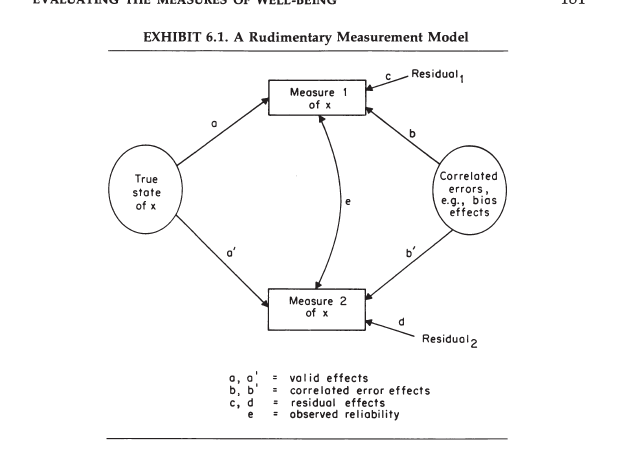
Exhibit 6.1 uses the graphical language of structural equation modelling to illustrate the measurement model. Here the oval on the left represents the true variation in well-being perceptions in a sample. The boxes in the middle represent two measures of well-being (e.g., two ratings on a delighted-terrible scale). The oval on the right reflects sources that produce systematic measurement error (e.g., halo bias). In this model, the observed correlation is the retest reliability of a single global measure and it is a function of the strength of the causal effects of the true variance (path a and a’) and the systematic measurement (b and b’) on the two measures.
The problem with this model is that there is only one observed correlation and two possible causal effects (assuming equal strength for a and a’, and b and b’). Thus, it is unclear how much of the reliable variance reflects actual variation in true well-being.
To make empirical claims about the validity of global well-being ratings, it is necessary to embed them in a network of variables that shows theoretically predicted relationships. Within a larger set of variables, the path from the construct to the observed measures may be identifiable (Cronbach & Meehl, 1955; Schimmack, 2019).
Estimates Derived from the July Data
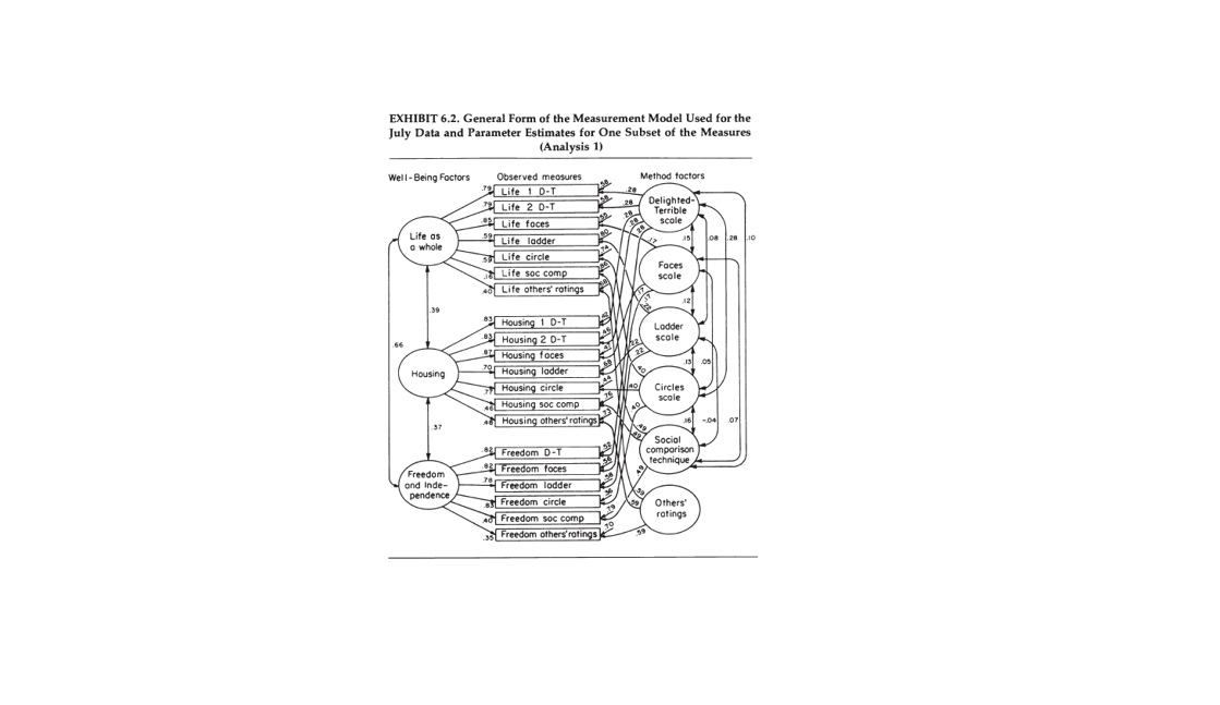
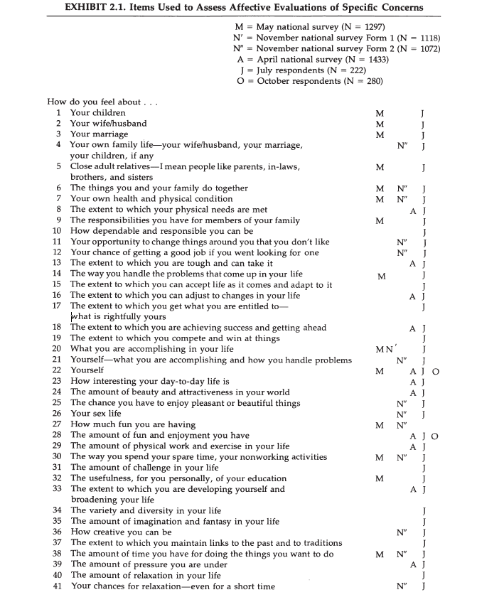
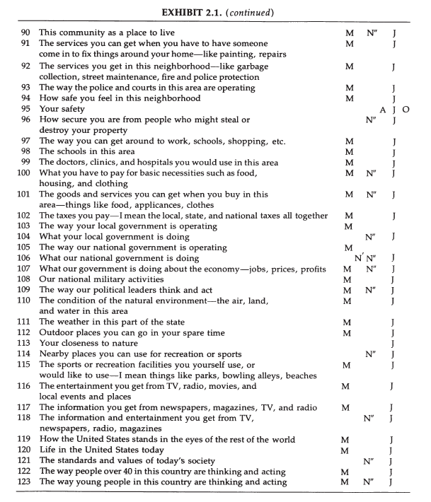
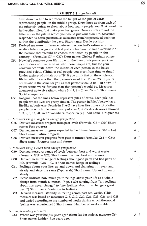
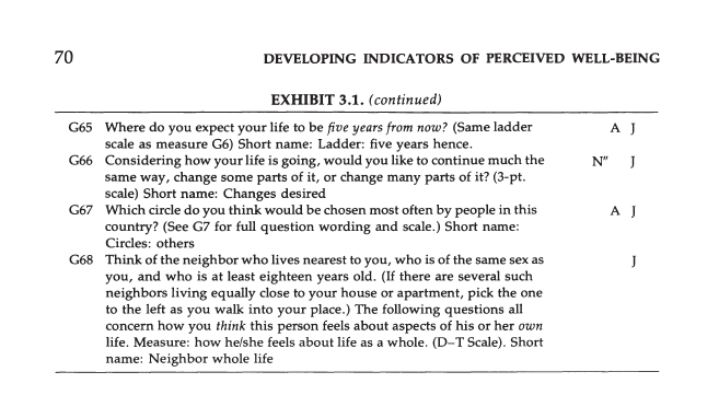
Scattered throughout the July questionnaire was a set of thirty-seven items that, when brought together for the purposes of the present analysis, forms a nearly complete six-by-six multimethod-multitrait matrix; i.e., a matrix in which six different “traits” (aspects of well-being) are assessed by each of six different methods. (p. 183)
The concerns were chosen to be well spread in the perceptual structure (as shown in Exhibit 2.2) and to include both domains and criteria. The following six aspects of well-being are represented: Life-as-a-whole, House or apartment, Spare-time activities, National government, Standard of living, and Independence or Freedom. The six measurement methods involve: self-ratings on the Delighted-Terrible, Faces, Circles, and Ladder Scales, the Social Comparison technique, and Ratings by others. (The exact wording of each of the concern-level items appears in Exhibit 2.1; see items 3D, 44, 85, 87, and 105. For descriptions of the six methods used to assess life-as-a-whole, see Exhibit 3.1, measures G1, G5, G6, G7, G13, and G54, these same methods were also used to assess the concern-level aspects. (p. 184).
Exhibit 6.2 shows the partial structural equation model for the global ratings and two domains. The key finding is that the correlations between residuals of the same rating scale tend to be rather small, while the validity coefficients are high. This seems to suggest that most of the reliable variance in global and domain measures is valid variance rather than systematic measurement error.
As much as I like Andrews and Withey’s work and recognize their contribution to well-being science in its infancy, I am disappointed by their discussion of the model.
Because the model shown in Exhibit 6.2 incorporates our theoretical expectations about how various phenomena influenced the validity and error components of the observed measures, because serious alternative theories have not come to our attention, and because the model in fact fits the data rather well (as will be described shortly), it seems reasonable to use it to estimate the validity and error components of the measures (p. 187)
On the basis of these results we infer that single item measures using the D-T, Faces, or Circles Scales to assess any of a wide range of different aspects of perceived well-being contain approximately 65 percent valid variance (p. 189).
Their own discussion of halo bias suggests that their model fails to account for systematic measurement error that is shared by different rating formats (Schimmack, , Böckenholt, & Reisenzein, 2002). It is well known that response sets have a negligible influence on ratings, but halo bias has a stronger influence.
It is important that the model actually includes measures that are based on the aggregated ratings of three informants that knew the respondent well (others’ rating). This makes the study a multi-method study that not only varies the response format, but also the rater. Other research has shown that halo bias is rather unique to a single rater (Anusic et al., 2009). Thus, halo bias cannot inflate correlations between respondents’ self-ratings and ratings by others. The problem is that a model with two-methods is unstable. It is only identified here because there are multiple self-ratings. In this case, halo bias can be hidden in higher loadings of the self-ratings on the true well-being factor than the other’ ratings. This is clearly the case. The loading for the informant ratings , as ratings by others’ are typically called, for global well-being is only .40, despite the fact that it is an average of three ratings and averaging increases validity. Based on the factor loadings, we can infer that the self-informant correlations are .4 * .8 = .32, which is in line with meta-analytic results from other studies (Schneider & Schimmack, 2009). A&W’s model gives the false impression that self-ratings are much more valid than informant ratings, but models that can test this assumption by using each informant as a separate method show that this is not the case (Zou et al., 2013). Thus, A&W’s work may have given a false impression about the validity of global well-being ratings. While they claimed that two-thirds of the variance is valid variance, other studies suggest it is only one-third, after taking halo bias into account.
A&W’s model shows high residual correlations among the three others’ ratings of life, housing, and freedom. They interpret this finding as evidence that halo bias has a strong influence on informant ratings.
The relatively high method effects in measures obtained from Others’ ratings is notable, but not terribly surprising. Since other people have less direct access to the respondents’ feelings than do the respondents themselves, one would expect substantially more “halo” in the Others’ ratings than in the respondents’ own ratings. This would be a reasonable explanation for the large amount of correlated error in these scores. (p. 189).
However, if these concerns are related to global well-being, but informant ratings have low loadings on the true factors, the model has to find another way to relate informant ratings of related to domains. The model is unable to test whether these correlations reflect bias or valid relationships. In contrast, other studies find no evidence that halo bias is considerably less present in self-ratings than in informant ratings (Anusic et al., 2009; Kim, Schimmack, & Oishi, 2012).
It is unfortunate that A&W and many researchers after them aggregated informant ratings, instead of treating informants as separate methods. As a result, 30 years of research failed to provide information about the amount of valid variance in self-ratings and informant ratings, leaving A&W’s estimate of 65% and 15% unquestioned. It was only in 2013, when Zou et al. (2013) showed that family members are as valid as the self in ratings of global well-being and that the proportions of variance are more equal around 30-40% valid variance for both. Self-ratings are only more valid when informant ratings are obtained from recent friends with less than two years of acquaintance (Schneider et al., 2010).
The low validity of informant ratings in A&W’s model led them to suggest that people are rather private about their true feelings about live.
What is of interest is that even people who the respondents felt knew them pretty well were in fact relatively poor judges of the respondents’ perceptions. This suggests that perceptions of well-being may be rather private matters. While people can-and did-give reasonably reliable answers (and, we estimate reasonably valid answers) regarding their affective evaluations of a wide range of life concerns, it would seem that they do not communicate their perceptions even to their friends and neighbors with much precision (p. 191).
While this may be true for neighbors, it is not true for family members. Moreover, other studies have found stronger correlations when informant ratings were aggregated across more informants and when informants are family members rather than neighbors (Schneider & Schimmack, 2009), and these stronger correlations have been used as evidence for the validity of self-ratings (Diener, Lucas, Schimmack, & Helliwell, 2009). Based on the same logic, A&W results would undermine the use of informant ratings as evidence of convergent validity of self-ratings.
There are several reasons why the modes validity of global well-being ratings has been ignored. First, it seems plausible that self-ratings are more valid because individuals have access to all of the relevant information. They know how things are going in their lives and they know what is important to them. In contrast, it is virtually certain that informants do not have access to all of the relevant information. However, these differences in accessibility of relevant information do not automatically ensure that self-ratings are more valid. This would only be the case if respondents are motivated to engage in an exhaustive search that retrieves all of the relevant information. This assumption has been questioned (Schwarz & Strack, 1999). Thus, we cannot simply assume that self-ratings are valid. The aim of validation research is to test this assumption. A&W’s model was unable to test it because they had several self-ratings and only one aggregated other-rating as indicators.
The second reason may be self-serving interest. The assumption that a single-item happiness rating can be used to measures something as complex and important as an individuals’ well-being makes these ratings very appealing for social scientists. If the assessment of well-being would require a complex set of questions about 20 life-domains with 10 criteria, it would be impossible to survey the well-being of nations and populations. The reason well-being is one of the most widely studied social constructs across several disciplines is that a single happiness item was easy to add to a survey.
DISTRIBUTIONS PRODUCED BY THE MORE VALID METHODS
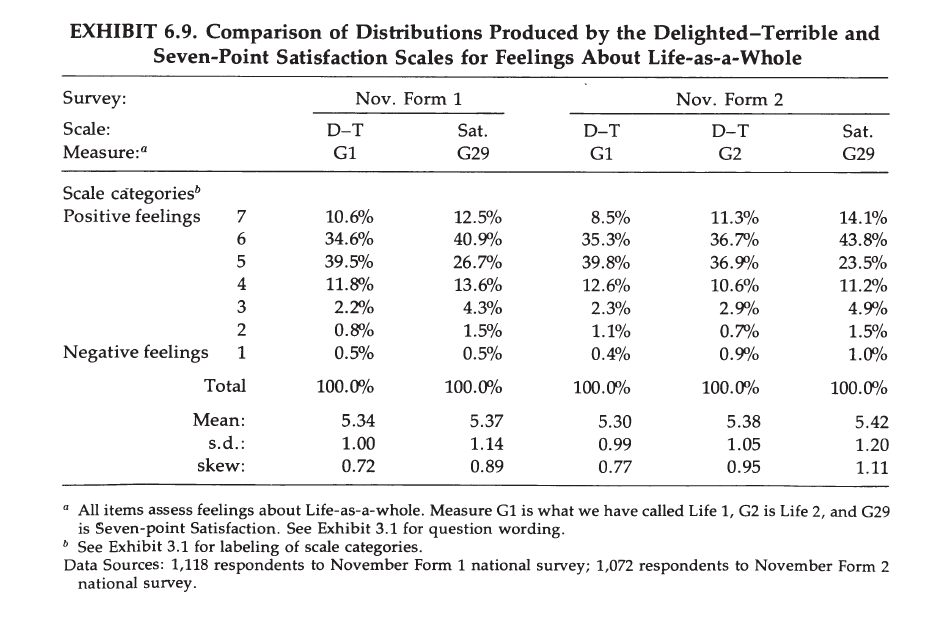
A&W also examine and care about the distribution of responses. They developed the delighted-terrible scale because they observed that even on a 7-point satisfaction scale responses clustered at the top.
Our data clearly show that the Delighted-Terrible Scale produces greater differentiation at the positive end of the scale than the seven-point Satisfaction Scale (p. 207).
However, the differences that they mention are rather small and both formats produce similar means.
RELATIONSHIPS BETWEEN MEASURES OF PERCEIVED WELL-BEING AND OTHER TYPES OF VARIABLES
a reasonably consistent and not very surprising pattern emerged. Nearly always, relationships were in the “expected” direction, and most were rather weak (p. 214).
However, these weak correlations were systematic and stronger when researchers expected stronger correlations.
“Where concerns had been judged relevant to the other items, the average correlation was .31; where staff members had been uncertain as to the concerns’ relevance, the average correlation was .25; and where concerns had been judged irrelevant the average correlation was .15″ (p. 214).
The problem is that A&W interpreted these results as evidence that perceived well-being is relatively independent of life conditions or actual behaviors.
Our general conclusion is that one will not usually find strong and direct relationships between measures of perceived well-being and reports of most life conditions or behaviors (p. 214).
This conclusion is partially based on the false inference that most of the variance in well-being ratings is valid variance. Another problem is that well-being is a broad construct and that a single behavior (e.g., sexual frequency; cf. Muise, Schimmack, & Impett, 2016) will only influence a small slice of the pizza of life. Other designs like twin studies or studies of spouses who are exposed to similar life circumstances are better suited to make claims about the importance of life conditions for well-being (Schimmack & Lucas, 2010). If differences in life circumstances do not explain variation in perceptions of well-being, what else could produce these differences? A&W do not address this question.
It would be naive to think that a person’s feelings about various aspects of life could be perfectly predicted by knowing only the characteristics of the person’s present environment. Developing adequate explanations for why people feel as they do about various life concerns would be a challenging undertaking in its own right. While we believe this could prove scientifically fruitful, such an investigation is not part of the work we are presently reporting.
This question became the focus of personality theories of well-being (Costa & McCrae, 1980; Diener, 1984) and it is now well-established that stable dispositions to experience more pleasure (positive affect) and less displeasure (negative affect) contribute to perceptions of well-being (Schimmack, Oishi, & Diener, 2002;
CHAPTER 7: Exploring the Dynamics of Evaluation
Explorations 1 and 2 examine how response categories of different formats correspond to each other.
EXPLORATION 3: HYPOTHETICAL FAMILY INCOMES AND AFFECTIVE EVALUATIONS ON THE D-T SCALE
This exploration examined response options on the delighted-terrible scale in relation to hypothetical income levels.
The dollar amounts would need to be translated into current dollar amounts to be meaningful. Nevertheless, it is surprising how small the gaps are even for the highest, delighted, category.
EXPLORATION 6: AN IMPLEMENTATION OF THE DOMAINS-BY-CRITERIA MODEL
Design of the Analysis and Measures Employed
A&W wrote items for each of the 48 cells in the 6 domains x 8 criteria matrix. They found that all items had small to moderate correlations with the global measure.
“The fortyeight correlations involved range from .13 to .41 with a mean of .20.”
Domain-criterion items were also more strongly correlated with judgments of the same domain than with other domains.
If the model is right, each concern-level variable should tend to have higher relationships with the cell variables that are assumed to influence it than with other cell variables. This expectation also proves to be supported by the data. For the domains, the average of the forty-eight correlations with “relevant” cell variables is .48 (as noted previously) while the average of the 240 correlations with “irrelevant” cell variables is .20 (p. 236).
For the criteria, a similar but somewhat smaller difference exists: The forty-eight correlations with “relevant” cell variables average .37, while the 320 correlations with “irrelevant” cell variables average .27. Furthermore, these differences are not reversed for any of the fourteen concern measures considered individually (p. 236).
Exhibit 7.5 shows regression weights from a multiple regression with (a) criteria as predictors (top) and with domains as predictors (bottom). At the top, the key criteria are fun and accomplishments. Standard of living matters only for evaluations of housing and national government, beauty for housing and neighbourhood. At the bottom, housing family and free time contribute to fun, and job and free time contribute to accomplishments. Free time probably does so by means of hobbies or volunteering. For life in general, fun and accomplishment (top) and housing, family, free time, and job are the key predictors.
EXPLORATION 7: COMPARISONS BETWEEN ONE’S OWN WELL-BEING AND THAT OF OTHERS
When Life-as-a-whole is being assessed, the consistent finding is that most people think they are better off than either other people in general (“all the adults in the U.S.”) or their nearest same-sexed neighbor. (p. 240).
This finding is probably just the typical better-than-average effect that is obtained for desirable traits. One explanation for it is that people do not overestimate themselves, but rather underestimate others, and do not sufficiently adjust the comparison. After all, if A&W are right we do not know much about the well-being of others, especially when we do not know them well.
Interestingly, the results switch for national government, which receives low ratings. So, here the adjustment problem works in the opposite direction and respondents underestimate how dissatisfied others are with the government.
EXPLORATION 8: JUDGMENTS OF THE “IMPORTANCE” OF CONCERNS
“One of the hypotheses with which we started was that the relative importance a person assigned to various life concerns should be taken into account when combining concern-level evaluations to predict feelings about Life-as-awhole. The hypothesis is based on the expectation that when forming evaluations of overall well-being people would give greater “weight” to those concerns they felt were important, and less weight to those they regarded as less significant. As described in chapter 4, a careful examination of this hypothesis showed it to be untrue.”
In one analysis we looked to see whether the mean importance assigned to a given concern bore any relationship to its association with feelings about Life-as- a-whole. If our original hypothesis had been correct, one would have expected a high relationship here; feelings about Life-as-a-whole would have had more to do with feelings about the important concerns than with feelings about the others. Using the data from our colleagues’ survey the answer was essentially “no.” Over ten concerns, the rank correlation between mean importance and the size of the simple bivariate relationship (measured by the eta statistic) was – .39: There was a modest tendency for the concerns that had higher relationships to Life-as-a-whole to be judged less important: When we performed the same analysis using a more complex multivariate relationship derived by holding constant the effects of all other nine concerns (measured by the beta statistic from Multiple classification Analysis), the rank correlation was + .15. A similar analysis in the July data produced a rank correlation of + .30 between the importance of concerns and the size of their (bivariate) relationships to the Life 3 measure. It seems clear that the mean importance assigned to a concern has little to do with the relationship between that concern and feelings about Life-as-a-whole (p. 243).
This is a puzzling finding and seems to undermine A&W’s bottom-up model of well-being perceptions. One problem is that Pearson correlations are sensitive to the amount of variance and the distribution of variables. For example, health could be important, but because it is important it is at high levels for most respondents. As a result, the Pearson correlation with perceived well-being would be low, which it actually is. A different kind of correlation coefficient or analysis would be needed for a better test of the hypothesis that more important domains are stronger predictors of well-being perceptions.
Further insight about the meaning of importance judgments emerged when we checked to see whether the importance assigned to a concern has anything to do with the position of the concern in the psychological structure. We compared the importance data for the ten concerns as assessed in our colleagues’ survey with the position of those concerns in the structural maps derived from our own national sample of May respondents (see Exhibit 2.4). There was a distinct tendency for concerns that were closer to Self and Family to receive higher importance ratings than those that were more remote (rho = .52). When the analysis was repeated using the importance of the concerns as judged by our July respondents, a parallel result emerged (rho = .43). Still a third version of the analysis took the importance of the concerns as judged by the July respondents and checked the location of the concerns in the plot derived from these same respondents (Exhibit 2.2). Here the relationship was somewhat higher (rho = .59). We conclude that importance ratings are substantially linked to the position of the concern in the perceptual structure, and that concerns that are seen as being closely associated with oneself and one’s family tend to be ranked as more important than others. (p. 244)
This is an interesting observation, but A&W do not elaborate further on it. Thus, it remains a mystery why respondents’ rate some domains as more important, but variation in these domains is not a stronger predictor of well-being evaluations.
END OF PART I
Conclusion
A&W provided a groundbreaking and exemplary examination of the construct validity of global well-being ratings. They presented a coherent theory that assumes global well-being judgments are integrative, mostly additive, evaluations of several life domains based on several criteria. Surprisingly, they found that weighing domains by importance did not improve predictions. They also tested a multi-trait-multi-method model to separate valid variance from method variance in well-being ratings. They concluded that two-thirds of the variance in self-ratings is valid, but only 15% of the variance in informant ratings are valid. Based on these results, they concluded that even a single global well-being rating is a valid measure of individuals’ true feelings about their lives, which we would rather call attitudes towards their lives, these days.
It is unfortunate that few well-being researchers have tried to build on A&W’s seminal work. To my knowledge, I am the only one who has fitted MTMM models to self-ratings and informant ratings of well-being to separate valid variance from systematic measurement error. Ironically, A&W’s impressive results may be the reason why further validation research has been neglected. However, A&W made some mistakes in their MTMM model and never explained the inconsistency between the bottom-up theory and their finding that importance weights do not improve prediction. Unfortunately, it is possible that their model was wrong and that a much larger portion of the variance in single-item well-being measures is method variance and that bottom-up effects on these measures are relatively weak and do not reflect the true importance of life circumstances for individuals’ well-being. Health is a particularly relevant domain. According to A&W’s results, variation in health satisfaction has relatively little unique effect on global well-being ratings. Does this really mean that health is unimportant? Does this mean that the massive increase in health spending over the past years is a waste of money? Or does it mean, global life evaluations are not as valid as we think they are and they fail to capture the relative importance of life domains for individuals’ well-being?
Here is a link to the manuscript, data, and MPLUS scripts for reproducibility. https://osf.io/mu7e6/
ABSTRACT
Greenwald et al. (1998) proposed that the IAT measures
individual differences in implicit social cognition. This claim requires evidence of construct validity.
I review the evidence and show that there is insufficient evidence for this
claim. Most important, I show that few
studies were able to test discriminant validity of the IAT as a measure of
implicit constructs. I examine discriminant validity in several multi-method
studies and find no or weak evidence for discriminant validity. I also show
that validity of the IAT as a measure of attitudes varies across constructs. Validity
of the self-esteem IAT is low, but estimates vary across studies. About 20% of the variance in the race IAT
reflects racial preferences. The highest validity is obtained for measuring
political orientation with the IAT (64% valid variance). Most of this valid variance stems from a
distinction between individuals with opposing attitudes, while reaction times
contribute less than 10% of variance in the prediction of explicit attitude
measures. In all domains, explicit
measures are more valid than the IAT, but the IAT can be used as a measure of
sensitive attitudes to reduce measurement error by using a multi-method
measurement model.
Despite its popularity, relatively little is known about the construct validity of the IAT.
As Cronbach (1989) pointed out, construct validation is better examined by independent experts than by authors of a test because “colleagues are especially able to refine the interpretation, as they compensate for blind spots and capitalize on their own distinctive experience” (p. 163).
It is of utmost importance to determine how much of the variance in IAT scores is valid variance and how much of the variance is due to measurement error, especially when IAT scores are used to provide individualized feedback.
There is also no consensus in the literature whether the IAT measures something different from explicit measures.
In conclusion, while there is general consensus to make a distinction between explicit measures and implicit measures, it is not clear what the IAT measures
To complicate matters further, the validity of the IAT may vary across attitude objects. After all the IAT is a method, just like Likert scales are a method, and it is impossible to say that a method is valid (Cronbach, 1971).
At present, relatively little is known about the contribution of these three parameters to observed correlations in hundreds of mono-method studies.
A Critical Review
of Greenwald et al.’s (1998) Original Article
In conclusion, the seminal IAT article introduced the IAT as a measure of implicit constructs that cannot be measured with explicit measures, but it did not really test this dual-attitude model.
Construct Validity in 2007
In conclusion, the 2007 review of construct validity revealed major psychometric challenges for the construct validity of the IAT, which explains why some researchers have concluded that the IAT cannot be used to measure individual differences (Payne et al., 2017). It also revealed that most studies were mono-method studies that could not examine convergent and discriminant validity
Cunningham, Preacher and Banaji (2001)
Another noteworthy finding is that a single factor accounted for correlations among all measures on the same occasion and across measurement occasions. This finding shows that there were no true changes in racial attitudes over the course of this two-month study. This finding is important because Cunningham et al.’s (2001) study is often cited as evidence that implicit attitudes are highly unstable and malleable (e.g., Payne et al., 2017). This interpretation is based on the failure to distinguish random measurement error and true change in the construct that is being measured (Anusic & Schimmack, 2016). While Cunningham et al.’s (2001) results suggest that the IAT is a highly unreliable measure, the results also suggest that the racial attitudes that are measured with the race IAT are highly stable over periods of weeks or months.
Bar-Anan & Vianello, 2018
this large study of construct validity also provides little evidence for the original claim that the IAT measures a new construct that cannot be measured with explicit measures, and confirms the estimate from Cunningham et al. (2001) that about 20% of the variance in IAT scores reflects variance in racial attitudes.
Greenwald et al. (2009)
“When entered after the self-report measures, the two implicit measures incrementally explained 2.1% of vote intention variance, p=.001, and when political conservativism was also included in the model, “the pair of implicit measures incrementally predicted only 0.6% of voting intention variance, p = .05.” (Greenwald et al., 2009, p. 247).
I tried to reproduce these results with the published correlation matrix and failed to do so. I contacted Anthony Greenwald, who provided the raw data, but I was unable to recreate the sample size of N = 1,057. Instead I obtained a similar sample size of N = 1,035. Performing the analysis on this sample also produced non-significant results (IAT: b = -.003, se = .044, t = .070, p = .944; AMP: b = -.014, se = .042, t = 0.344, p = .731). Thus, there is no evidence for incremental predictive validity in this study.
Axt (2018)
With N = 540,723 respondents, sampling error is very small, σ = .002, and parameter estimates can be interpreted as true scores in the population of Project Implicit visitors. A comparison of the factor loadings shows that explicit ratings are more valid than IAT scores. The factor loading of the race IAT on the attitude factor once more suggests that about 20% of the variance in IAT scores reflects racial attitudes
Falk, Heine, Zhang, and Hsu (2015)
Most important, the self-esteem IAT and the other implicit measures have low and non-significant loadings on the self-esteem factor.
Bar-Anan & Vianello (2018)
Thus, low validity contributes considerably to low observed correlations between IAT scores and explicit self-esteem measures.
Bar-Anan & Vianello (2018) – Political Orientation
More important, the factor loading of the IAT on the implicit factor is much higher than for self-esteem or racial attitudes, suggesting over 50% of the variance in political orientation IAT scores is valid variance, π = .79, σ = .016. The loading of the self-report on the explicit ratings was also higher, π = .90, σ = .010
Variation of Implicit – Explicit Correlations Across Domains
This suggests that the IAT is good in classifying individuals into opposing groups, but it has low validity of individual differences in the strength of attitudes.
What Do IATs Measure?
The present results suggest that measurement error alone is often sufficient to explain these low correlations. Thus, there is little empirical support for the claim that the IAT measures implicit attitudes that are not accessible to introspection and that cannot be measured with self-report measures.
For 21 years the lack of discriminant validity has been overlooked because psychologists often fail to take measurement error into account and do not clearly distinguish between measures and constructs.
In the future, researchers need to be more careful when they make claims about constructs based on a single measure like the IAT because measurement error can produce misleading results.
Researchers should avoid terms like implicit attitude or implicit preferences that make claims about constructs simply because attitudes were measured with an implicit measure
Recently, Greenwald and Banaji (2017) also expressed concerns about their earlier assumption that IAT scores reflect unconscious processes. “Even though the present authors find themselves occasionally lapsing to use implicit and explicit as if they had conceptual meaning, they strongly endorse the empirical understanding of the implicit– explicit distinction” (p. 862).
How
Well Does the IAT Measure What it Measures?
Studies with the IAT can be divided into applied studies (A-studies) and basic studies (B-studies). B-studies employ the IAT to study basic psychological processes. In contrast, A-studies use the IAT as a measure of individual differences. Whereas B-studies contribute to the understanding of the IAT, A-studies require that IAT scores have construct validity. Thus, B-studies should provide quantitative information about the psychometric properties for researchers who are conducting A-studies. Unfortunately, 21 years of B-studies have failed to do so. For example, after an exhaustive review of the IAT literature, de Houwer et al. (2009) conclude that “IAT effects are reliable enough to be used as a measure of individual differences” (p. 363). This conclusion is not helpful for the use of the IAT in A-studies because (a) no quantitative information about reliability is given, and (b) reliability is necessary but not sufficient for validity. Height can be measured reliably, but it is not a valid measure of happiness.
This article provides the first quantitative information about validity of three IATs. The evidence suggests that the self-esteem IAT has no clear evidence of construct validity (Falk et al., 2015). The race-IAT has about 20% valid variance and even less valid variance in studies that focus on attitudes of members from a single group. The political orientation IAT has over 40% valid variance, but most of this variance is explained by group-differences and overlaps with explicit measures of political orientation. Although validity of the IAT needs to be examined on a case by case basis, the results suggest that the IAT has limited utility as a measurement method in A-studies. It is either invalid or the construct can be measured more easily with direct ratings.
Implications for the Use of IAT scores in Personality Assessment
I suggest to replace the reliability coefficient with the validity coefficient. For example, if we assume that 20% of the variance in scores on the race IAT is valid variance, the 95%CI for IAT scores from Project Implicit (Axt, 2018), using the D-scoring method, with a mean of .30 and a standard deviation of.46 ranges from -.51 to 1.11. Thus, participants who score at the mean level could have an extreme pro-White bias (Cohen’s d = 1.11/.46 = 2.41), but also an extreme pro-Black Bias (Cohen’s d = -.51/.46 = -1.10). Thus, it seems problematic to provide individuals with feedback that their IAT score may reveal something about their attitudes that is more valid than their beliefs.
Conclusion
Social psychologists have always distrusted self-report, especially for the measurement of sensitive topics like prejudice. Many attempts were made to measure attitudes and other constructs with indirect methods. The IAT was a major breakthrough because it has relatively high reliability compared to other methods. Thus, creating the IAT was a major achievement that should not be underestimated because the IAT lacks construct validity as a measure of implicit constructs. Even creating an indirect measure of attitudes is a formidable feat. However, in the early 1990s, social psychologists were enthralled by work in cognitive psychology that demonstrated unconscious or uncontrollable processes (Greenwald & Banaji, 1995). Implicit measures were based on this work and it seemed reasonable to assume that they might provide a window into the unconscious (Banaji & Greenwald, 2013). However, the processes that are involved in the measurement of attitudes with implicit measures are not the personality characteristics that are being measured. There is nothing implicit about being a Republican or Democrat, gay or straight, or having low self-esteem. Conflating implicit processes in the measurement of attitudes with implicit personality constructs has created a lot of confusion. It is time to end this confusion. The IAT is an implicit measure of attitudes with varying validity. It is not a window into people’s unconscious feelings, cognitions, or attitudes.
This article was published in a special issue in the European Journal of Personality Psychology. It examines the unresolved issue of validating psychological measures fro the perspective of a multi-method approach (Campbell & Fiske, 1959), using structural equation modeling.
I think it provides a reasonable alternative to the current interest in modeling residual variance in personality questionnaires (network perspective) and solves the problems of manifest personality measures that are confounded by systematic measurement error.
Although latent variable models of multi-method data have been used in structural analyses (Biesanz & West, 2004; deYoung, 2006), these studies have rarely been used to estimate validity of personality measures. This article shows how this can be done and what assumptions need to be made to interpret latent factors as variance in true personality traits.
Hopefully, sharing this article openly on this blog can generated some discussion about the future of personality measurement in psychology.
What Multi-Method Data Tell Us About
Construct Validity
ULRICH SCHIMMACK*
University of Toronto Mississauga, Canada
European Journal of Personality
Eur. J. Pers. 24: 241–257 (2010)
DOI: 10.1002/per.771 [for original article]
Abstract
Structural equation modelling of multi-method data has become a popular method to
examine construct validity and to control for random and systematic measurement error in personality measures. I review the essential assumptions underlying causal models of
multi-method data and their implications for estimating the validity of personality
measures. The main conclusions are that causal models of multi-method data can be
used to obtain quantitative estimates of the amount of valid variance in measures of
personality dispositions, but that it is more difficult to determine the validity of personality measures of act frequencies and situation-specific dispositions.
Key words: statistical methods; personality scales and inventories; regression methods;
history of psychology; construct validity; causal modelling; multi-method; measurement
INTRODUCTION
Fifty years ago, Campbell and Fiske (1959) published the groundbreaking article
Convergent and Discriminant Validation by the Multitrait-Multimethod Matrix.With close to 5000 citations (Web of Science, February 1, 2010), it is the most cited article in
Psychological Bulletin. The major contribution of this article was to outline an empirical
procedure for testing the validity of personality measures. It is difficult to overestimate the importance of this contribution because it is impossible to test personality theories
empirically without valid measures of personality.
Despite its high citation count, Campbell and Fiske’s work is often neglected in
introductory textbooks, presumably because validation is considered to be an obscure and complicated process (Borsboom, 2006). Undergraduate students of personality psychology learn little more than the definition of a valid measure as a measure that measures what it is supposed to measure.
However, they are not taught how personality psychologists validate their measures. One might hope that aspiring personality researchers learn about Campbell and Fiske’s multi-method approach during graduate school. Unfortunately, even handbooks dedicated to research methods in personality psychology pay relatively little attention to Campbell and Fiske’s (1959) seminal contribution (John & Soto, 2007; Simms & Watson, 2007). More importantly, construct validity is often introduced in qualitative terms.
In contrast, when Cronbach and Meehl (1955) introduced the concept of construct validity, they proposed a quantitative definition of construct validity as the proportion of construct-related variance in the observed variance of a personality measure. Although the authors noted that it would be difficult to obtain precise estimates of construct validity coefficients (CVCs), they stressed the importance of estimating ‘as definitely as possible the degree of validity the test is presumed to have’ (p. 290).
Campbell and Fiske’s (1959) multi-method approach paved the way to do so. Although Campbell and Fiske’s article examined construct validity qualitatively, subsequent developments in psychometrics allowed researchers to obtain quantitative estimates of construct validity based on causal models of multi-method data (Eid, Lischetzke, Nussbeck, & Trierweiler, 2003; Kenny & Kashy, 1992). Research articles in leading personality journals routinely report these estimates (Biesanz & West, 2004; DeYoung, 2006; Diener, Smith, & Fujita, 1995), but a systematic and accessible introduction to causal models of multi-method data is lacking.
The main purpose of this paper is to explain how causal models of multi-method data can be used to obtain quantitative estimates of construct validity and which assumptions these models make to yield accurate estimates.
I prefer the term causal model to the more commonly used term structural equation model because I interpret latent variables in these models as unobserved, yet real causal forces that produce variation in observed measures (Borsboom, Mellenbergh,&
van Heerden, 2003). I make the case below that this realistic interpretation of latent factors is necessary to use multi-method data for construct validation research because the assumption of causality is crucial for the identification of latent variables with construct variance (CV).
Campbell and Fiske (1959) distinguished absolute and relative (construct) validity. To
examine relative construct validity it is necessary to measure multiple traits and to look for evidence of convergent and discriminant validity in a multi-trait-multi-method matrix (Simms &Watson, 2007). However, to examine construct validity in an absolute sense, it is only necessary to measure one construct with multiple methods.
In this paper, I focus on convergent validity across multiple measures of a single construct because causal models of multi-method data rely on convergent validity alone to examine construct validity.
As discussed in more detail below, causal models of multi-method data estimate
construct validity quantitatively with the factor loadings of observed personality measures on a latent factor (i.e. an unobserved variable) that represents the valid variance of a construct. The amount of valid variance in a personality measure can be obtained by squaring its factor loading on this latent factor. In this paper, I use the terms construct validity coefficient (CVC) to refer to the factor loading and the term construct variance (CV) for the amount of valid variance in a personality measure.
Validity
A measure is valid if it measures what it was designed to measure. For example, a
thermometer is a valid measure of temperature in part because the recorded values covary with humans’ sensory perceptions of temperature (Cronbach & Meehl, 1955). A modern thermometer is a more valid measure of temperature than humans’ sensory perceptions, but the correlation between scores on a thermometer and humans’ sensory perceptions is necessary to demonstrate that a thermometer measures temperature. It would be odd to claim that highly reliable scores recorded by an expensive and complicated instrument measure temperature if these scores were unrelated to humans’ everyday perceptions of temperature.
The definition of validity as a property of a measure has important implications for
empirical tests of validity. Namely, researchers first need a clearly defined construct before they can validate a potential measure of the construct. For example, to evaluate a measure of anxiety researchers first need to define anxiety and then examine the validity of a measure as a measure of anxiety. Although the importance of clear definitions for construct validation research may seem obvious, validation research often seems to work in the opposite direction; that is, after a measure has been created psychologists examine what it measures.
For example, the widely used Positive Affect and Negative Affect Schedule (PANAS) has two scales named Positive Affect (PA) and Negative Affect (NA). These scales are based on exploratory factor analyses of mood ratings (Watson, Clark, & Tellegen, 1988). As a result, Positive Affect and Negative Affect are merely labels for the first two VARIMAX rotated principal components that emerged in these analyses. Thus, it is meaningless to examine whether the PANAS scales are valid measures of PA and NA. They are valid measures of PA and NA by definition because PA and NA are mere labels of the two VARIMAX rotated principal components that emerge in factor analyses of mood ratings.
A construct validation study would have to start with an a priori definition of Positive Affect and Negative Affect that does not refer to the specific measurement procedure that was used to create the PANAS scales. For example, some researchers have
defined Positive Affect and Negative Affect as the valence of affective experiences and
have pointed out problems of the PANAS scales as measures of pleasant and unpleasant
affective experiences (see Schimmack, 2007, for a review).
However, the authors of the PANAS do not view their measure as a measure of hedonic valence. To clarify their position, they proposed to change the labels of their scales from Positive Affect and Negative Affect to Positive Activation and Negative Activation (Watson,Wiese, Vaidya, & Tellegen, 1999). The willingness to change labels indicates that PANAS scales do not measure a priori defined constructs and as a result there is no criterion to evaluate the construct validity of the PANAS scales.
The previous example illustrates how personality measures assume a life of their own
and implicitly become the construct; that is, a construct is operationally defined by the
method that is used to measure it (Borsboom, 2006). A main contribution of Cambpell and Fiske’s (1959) article was to argue forcefully against operationalism and for a separation of constructs and methods. This separation is essential for validation research because validation research has to allow for the possibility that some of the observed variance is invalid.
Other sciences clearly follow this approach. For example, physics has clearly defined
concepts such as time or temperature. Over the past centuries, physicists have developed
increasingly precise ways of measuring these concepts, but the concepts have remained the same. Modern physics would be impossible without these advances in measurement.
However, psychologists do not follow this model of more advanced sciences. Typically, a
measure becomes popular and after it becomes popular it is equated with the construct. As a result, researchers continue to use old measure and rarely attempt to create better
measures of the same construct. Indeed, it is hard to find an example, in which one measure of a construct has replaced another measure of the same construct based on an empirical comparison of the construct validity of competing measures of the same construct (Grucza & Goldberg, 2007).
One reason for the lack of progress in the measurement of personality constructs could
be the belief that it is impossible to quantify the validity of a measure. If it were impossible to quantify the validity of a measure, then it also would be impossible to say which of two measures is more valid. However, causal models of multi-method data produce quantitative estimates of validity that allow comparisons of the validity of different measures.
One potential obstacle for construct validation research is the need to define
psychological constructs a priori without reference to empirical data. This can be difficult for constructs that make reference to cognitive processes (e.g. working memory capacity) or unconscious motives (implicit need for power). However, the need for a priori definitions is not a major problem in personality psychology. The reason is that everyday language provides thousands of relatively well-defined personality constructs (Allport & Odbert, 1936). In fact, all measures in personality psychology that are based on the lexical hypothesis assume that everyday concepts such as helpful or sociable are meaningful personality constructs. At least with regard to these relatively simple constructs, it is possible to test the construct validity of personality measures. For example, it is possible to examine whether a sociability scale really measures sociability and whether a measure of helpfulness really measures helpfulness.
Convergent validity
I start with a simple example to illustrate how psychologists can evaluate the validity of a
personality measure. The concept is people’s weight.Weight can be defined as ‘the vertical force exerted by a mass as a result of gravity’ (wordnet.princeton.edu). In the present case, only the mass of human adults is of interest. The main question, which has real practical significance in health psychology (Kroh, 2005), is to examine the validity of self-report measures of weight because it is more economical to use self-reports than to weigh people with scales.
To examine the validity of self-reported weight as a measure of actual weight, it is
possible to obtain self-reports of weight and an objective measure of weight from the same individuals. If self-reports of weight are valid, they should be highly correlated with the objective measure of weight. In one study, participants first reported their weight before their weight was objectively measured with a scale several weeks later (Rowland, 1990). The correlation in this study was r (N =11,284) =.98. The implications of this finding for the validity of self-reports of weight depend on the causal processes that underlie this correlation, which can be examined by means of causal modelling of correlational data.
It is well known that a simple correlation does not reveal the underlying causal process,
but that some causal process must explain why a correlation was observed (Chaplin, 2007). Broadly speaking, a correlation is determined by the strength of four causal effects, namely, the effect of observed variable A on observed variable B, the effect of observed variable B on observed variable A, and the effects of an unobserved variable C on observed variable A and on observed variable B.
In the present example, the observed variables are the self-reported weights and those recorded by a scale. To make inferences about the validity of self-reports of weight it is necessary to make assumptions about the causal processes that produce a correlation between these two methods. Fortunately, it is relatively easy to do so in this example. First, it is fairly certain that the values recorded by a scale are not influenced by individuals’ self-reports. No matter how much individuals insist that the scale is wrong, it will not change its score. Thus, it is clear that the causal effect of self-reports on
the objective measure is zero. It is also clear that self-reports of weight in this study were
not influenced by the objective measurement of weight in this study because self-reports
were obtained weeks before the actual weight was measured. Thus, the causal effect of the objectively recorded scores on self-rating is also zero. It follows that the correlation of r =.98 must have been produced by a causal effect of an unobserved third variable. A
plausible third variable is individuals’ actual mass. It is their actual mass that causes the
scale to record a higher or lower value and their actual mass also caused them to report a specific weight. The latter causal effect is probably mediated by prior objective
measurements with other scales, and the validity of these scales would influence the
validity of self-reports among other factors (e.g. socially desirable responding). In combination, the causal effects of actual mass on self-reports and on the scale produce the observed correlation of r =.98. This correlation is not sufficient to determine how strong the effects of weight on the two measures are. It is possible that the scale was a perfect measure of weight. In this case, the correlation between weight and the values recorded by the scale is 1. It follows, that the size of the effect of weight on self-reports of weight (or the factor loading of self-reported weight on the weight factor) has to be r =.98 to produce the observed correlation of r =.98 (1 *.98 = .98). In this case, the CVC of the self-report measure of weight would be .98. However, it is also possible that the scale is a slightly imperfect measure of weight. For example, participants may not have removed their shoes before stepping on the scale and differences in the weight of shoes (e.g. boots versus sandals) could have produced measurement error in the objective measure of individuals’ true weight. It is also possible that changes in weight over time reduce the validity of objective scores as a validation criterion for self-ratings several weeks earlier. In this case, the estimate underestimates the validity of self-ratings.
In the present context, the reasons for the lack of perfect convergent validity are irrelevant. The main point of this example was to illustrate how the correlation between two independent measures of the same construct can be used to obtain quantitative estimates of the validity of a personality measure. In this example, a conservative estimate of the CVC of self-reported weight as a measure of weight is .98 and the estimated amount of CVin the self-report measure is 96% (.98^2 = .96).
The example of self-reported weight was used to establish four important points about
construct validity. First, the example shows that convergent validity is sufficient to examine construct validity. The question of how self-reports of weight are related to measures of other constructs (e.g. height, social desirable responding) can be useful to examine sources of measurement error, but correlations with measures of other constructs are not needed to estimate CVCs. Second, empirical tests of construct validity do not have to be an endless process without clear results (Borsboom, 2006). At least for some self-report measures it is possible to provide a meaningful answer to the question of their validity. Third, validity is a quantitative construct. Qualitative conclusions that a measure is valid because validity is not zero (CVC>0, p<.05) or that a measure is invalid because validity is not perfect (CVC<1.0, p<.05) are not very helpful because most measures are valid and invalid (0<CVC<1). As a result, qualitative reviews of validity studies are often the source of fruitless controversies (Schimmack & Oishi, 2005). The validity of personality measures should be estimated quantitatively like other psychometric properties such as reliability coefficients, which are routinely reported in research articles (Schmidt & Hunter, 1996).
Validity is more important than reliability because reliable and invalid measures are
potentially more dangerous than unreliable measures (Blanton & Jaccard, 2006). Moreover, it is possible that a less reliable measure is more valid than a more reliable measure if the latter measure is more strongly contaminated by systematic measurement error (John & Soto, 2007). A likely explanation for the emphasis on reliability is the common tendency to equate constructs with measures. If a construct is equated with a measure, only random error can undermine the validity of a measure. The main contribution of Campbell and Fiske (1959) was to point out that systematic measurement error can also threaten the validity of personality measures. As a result, high reliability is insufficient evidence for the validity of a personality measure (Borsboom & Mellenbergh, 2002).
The third point illustrated in this example is that tests of convergent validity require
independent measures. Campbell and Fiske (1959) emphasized the importance of
independent measures when they defined convergent validity as the correlation between ‘maximally different methods’ (p. 83). In a causal model of multi-method data the independence assumption implies that the only causal effects that produce a correlation between two measures of the same construct are the causal effect of the construct on the two measures. This assumption implies that all the other potential causal effects that can produce correlations among observed measures have an effect size of zero. If this assumption is correct, the shared variance across independent methods represents CV. It is then possible to estimate the proportion of the shared variance relative to the total observed variance of a personality measure as an estimate of the amount of CV in this measure. For example, in the previous example I assumed that actual mass was the only causal force that contributed to the correlation between self-reports of weight and objective scale scores. This assumption would be violated if self-ratings were based on previous measurements with objective scales (which is likely) and objective scales share method variance that does not reflect actual weight (which is unlikely). Thus, even validation studies with objective measures implicitly make assumptions about the causal model underling these correlations.
In sum, the weight example illustrated how a causal model of the convergent validity
between two measures of the same construct can be used to obtain quantitative estimates of the construct validity of a self-report measure of a personality characteristic. The following example shows how the same approach can be used to examine the construct validity of measures that aim to assess personality traits without the help of an objective measure that relies on well-established measurement procedures for physical characteristics like weight.
CONVERGENT VALIDITY OF PERSONALITY MEASURES
A Hypothetical Example
I use helpfulness as an example. Helpfulness is relatively easy to define as ‘providing
assistance or serving a useful function’ (wordnetweb.princeton.edu/perl/webwn). Helpful can be used to describe a single act or an individual. If helpful is used to describe a single act, helpful is not only a characteristic of a person because helping behaviour is also influenced by situational factors and interactions between personality and situational factors. Thus, it is still necessary to provide a clearer definition of helpfulness as a personality characteristic before it is possible to examine the validity of a personality measure of helpfulness.
Personality psychologists use trait concepts like helpful in two different ways. The most
common approach is to define helpful as an internal disposition. This definition implies
causality. There are some causal factors within an individual that make it more likely for
this individual to act in a helpful manner than other individuals. The alternative approach is to define helpfulness as the frequency with which individuals act in a helpful manner. An individual is helpful if he or she acted in a helpful manner more often than other people. This approach is known as the act frequency approach. The broader theoretical differences between these two approaches are well known and have been discussed elsewhere (Block, 1989; Funder, 1991; McCrae & Costa, 1995). However, the implications of these two definitions of personality traits for the interpretation of multi-method data have not been discussed. Ironically, it is easier to examine the validity of personality measures that aim to assess internal dispositions that are not directly observable than to do so for personality measures that aim to assess frequencies of observable acts. This is ironic because intuitively it seems to be easier to count the frequency of observable acts than to measure unobservable internal dispositions. In fact, not too long ago some psychologists doubted that internal dispositions even exist (cf. Goldberg, 1992).
The measurement problem of the act frequency approach is that it is quite difficult to
observe individuals’ actual behaviours in the real world. For example, it is no trivial task to establish how often John was helpful in the past month. In comparison it is relatively easy to use correlations among multiple imperfect measures of observable behaviours to make inferences about the influence of unobserved internal dispositions on behaviour.
Figure 1. Theoretical model of multi-method data. Note. T = trait (general disposition); AF-c, AF-f, AF-s = act frequencies with colleague, friend and spouse; S-c, S-f, S-s =situational and person x situation interaction effects on act frequencies; R-c, R-f, R-s = reports by colleague, friend and spouse; E-c, E-f, E-s =errors in reports by
colleague, friend and spouse.
Figure 1 illustrates how a causal model of multi-method data can be used for this purpose. In Figure 1, an unobserved general disposition to be helpful influences three observed measures of helpfulness. In this example, the three observed measures are informant ratings of helpfulness by a friend, a co-worker and a spouse. Unlike actual informant ratings in personality research, informants in this hypothetical example are only asked to report how often the target helped them in the past month. According to Figure 1, each informant report is influenced by two independent factors, namely, the actual frequency of helpful acts towards the informant and (systematic and random) measurement error in the reported frequencies of helpful acts towards the informant. The actual frequency of helpful acts is also influenced by two independent factors. One factor represents the general disposition to be helpful that influences helpful behaviours across situations. The other factor represents situational factors and person-situation interaction effects. To fully estimate all coefficients in this model (i.e. effect sizes of the postulated causal effects), it would be necessary to separate measurement error and valid variance in act frequencies.
This is impossible if, as in Figure 1, each act frequency is measured with a single method,
namely, one informant report. In contrast, the influence of the general disposition is
reflected in all three informant reports. As a result, it is possible to separate the variance due to the general disposition from all other variance components such as random error,
systematic rating biases, situation effects and personsituation interaction effects. It is
then possible to determine the validity of informant ratings as measures of the general
disposition, but it is impossible to (precisely) estimate the validity of informant ratings as
measures of act frequencies because the model cannot distinguish reporting errors from
situational influences on helping behaviour.
The causal model in Figure 1 makes numerous independence assumptions that specify
Campbell and Fiske’s (1959) requirement that traits should be assessed with independent
methods. First, the model assumes that biases in ratings by one rater are independent of
biases in ratings by other raters. Second, it assumes that situational factors and
person by situation interaction effects that influence helping one informant are independent of the situational and personsituation factors that influence helping other informants. Third, it assumes that rating biases are independent of situation and person by situation interaction effects for the same rater and across raters. Finally, it assumes that rating biases and situation effects are independent of the global disposition. In total, this amounts to 21 independence assumptions (i.e. Figure 1 includes seven exogeneous variables, that is, variables that do not have an arrow pointing at them, which implies 21 (7×6/2) relationships that the model assumes to be zero). If these independence assumptions are correct, the correlations among the three informant ratings can be used to determine the variation in the unobserved personality disposition to be helpful with perfect validity. This variance can then be used like the objective measure of weight in the previous example as the validation criterion for personality measures of the general
disposition to be helpful (e.g. self-ratings of general helpfulness). In sum, Figure 1
illustrates that a specific pattern of correlations among independent measures of the same construct can be used to obtain precise estimates of the amount of valid variance in a single measure.
The main challenge for actual empirical studies is to ensure that the methods in a multi-method model fulfill the independence assumptions. The following examples demonstrate the importance of the neglected independence assumption for the correct interpretation of causal models of multi-method data. I also show how researchers can partially test the independence assumption if sufficient methods are available and how researchers can estimate the validity of personality measures that aggregate scores from independent methods. Before I proceed, I should clarify that strict independence of methods is unlikely, just like other null-hypotheses are likely to be false. However, small violations of the independence assumption will only introduce small biases in estimates of CVCs.
Example 1: Multiple response formats
The first example is a widely cited study of the relation between Positive Affect and
Negative Affect (Green, Goldman,&Salovey, 1993). I chose this paper because the authors
emphasized the importance of a multi-method approach for the measurement of affect,
while neglecting Campbell and Fiske’s requirement that the methods should be maximally different. A major problem for any empirical multi-method study is to find multiple independent measures of the same construct. The authors used four self-report measures with different response formats for this purpose. However, the variation of response formats can only be considered a multi-method study, if one assumes that responses on one response format are independent of responses on the other response formats so that correlations across response formats can only be explained by a common causal effect of actual momentary affective experiences on each response format. However, the validity of all self-report measures depends on the ability and willingness of respondents to report their experiences accurately. Violations of this basic assumption introduce shared method variance among self-ratings on different response formats. For example, socially desirable responding can inflate ratings of positive experiences across response formats. Thus, Green et al.’s (1993) study assumed rather than tested the validity of self-ratings of momentary affective experiences. At best, their study was able to examine the contribution of stylistic tendencies in the use of specific response formats to variance in mood ratings, but these effects are known to be small (Schimmack, Bockenholt, & Reisenzein, 2002). In sum, Green et al.’s (1993) article illustrates the importance of critically examining the similarity of methods in a multi-method study. Studies that use multiple self-report measures that vary response formats, scales, or measurement occasions should not be considered multi-method studies that can be used to examine construct validity.
Example 2: Three different measures
The second example of a multi-method study also examined the relation between Positive Affect and Negative Affect (Diener et al., 1995). However, it differs from the previous example in two important ways. First, the authors used more dissimilar methods that are less likely to violate the independence assumption, namely, self-report of affect in the past month, averaged daily affect ratings over a 6 week period and averaged ratings of general affect by multiple informants. Although these are different methods, it is possible that these methods are not strictly independent. For example, Diener et al. (1995) acknowledge that all three measures could be influenced by impression management. That is, retrospective and daily self-ratings could be influenced by social desirable responding, and informant ratings could be influenced by targets’ motivation to hide negative emotions from others. A common influence of impression management on all three methods would inflate validity estimates of all three methods.
For this paper, I used Diener et al.’s (1995) multi-method data to estimate CVCs for the
three methods as measures of general dispositions that influence people’s positive and
negative affective experiences. I used the data from Diener et al.’s (1995) Table 15 that are reproduced in Table 1. I used MPLUS5.1 for these analyses and all subsequent analyses (Muthen & Muthen, 2008). I fitted a simple model with a single latent variable that represents a general disposition that has causal effects on the three measures. Model fit was perfect because a model with three variables and three parameters has zero degrees of freedom and can perfectly reproduce the observed pattern of correlations. The perfect fit implies that CVC estimates are unbiased if the model assumptions are correct, but it also implies that the data are unable to test model assumptions.
These results suggest impressive validity of self-ratings of affect (Table 2). In contrast,
CVC estimates of informant ratings are considerably lower, despite the fact that informant ratings are based on averages of several informants. The non-overlapping confidence intervals for self-ratings and informant ratings indicate that this difference is statistically significant. There are two interpretations of this pattern. On the one hand, it is possible that informants are less knowledgeable about targets’ affective experiences. After all, they do not have access to information that is only available introspectively. However, this privileged information does not guarantee that self-ratings are more valid because individuals only have privileged information about their momentary feelings in specific situations rather than the internal dispositions that influence these feelings. On the other hand, it is possible that retrospective and daily self-ratings share method variance and do not fulfill the independence assumption. In this case, the causal model would provide inflated estimates of the validity of self-ratings because it assumes that stronger correlations between retrospective and daily self-ratings reveal higher validity of these methods, when in reality the higher correlation is caused by shared method effects. A study with three methods is unable to test these alternative explanations.
Example 3: Informants as multiple methods
One limitation of Diener et al.’s (1995) study was the aggregation of informant ratings.
Although aggregated informant ratings provide more valid information than ratings by a
single informant, the aggregation of informant ratings destroys valuable information about the correlations among informant ratings. The example in Figure 1 illustrated that ratings by multiple informants provide one of the easiest ways to measure dispositions with multiple methods because informants are more likely to base their ratings on different situations, which is necessary to reveal the influence of internal dispositions.
Example 3 shows how ratings by multiple informants can be used in construct validation research. The data for this example are based on multi-method data from the Riverside Accuracy Project (Funder, 1995; Schimmack, Oishi, Furr, & Funder, 2004). To make the CVC estimates comparable to those based on the previous example, I used scores on the depression and cheerfulness facets of the NEO-PI-R (Costa&McCrae, 1992). These facets are designed to measure affective dispositions. The multi-method model used self-ratings and informant ratings by parents, college friends and hometown friends as different methods.
Table 3 shows the correlation matrices for cheerfulness and depression. I first fitted a causal model that assumed independence of all methods to the data. The model also included sum scores of observed measures to examine the validity of aggregated informant ratings and an aggregated measure of all four raters (Figure 2). Model fit was evaluated using standard criteria of model fit, namely, comparative fit index (CFI)>.95, root mean square error of approximation (RMSEA)<.06 and standardized
root mean residuals (SRMR)<.08.
Neither cheerfulness, chi2 (df =2, N =222) = 11.30, p<.01, CFI =.860, RMSEA =.182, SRMR = .066, nor depression, chi2 (df =2, N = 222) = 8.31, p =.02, CFI =. 915, RMSEA = .150, SRMR =.052, had acceptable CFI and RSMEA values.
One possible explanation for this finding is that self-ratings are not independent of informant ratings because self-ratings and informant ratings could be partially based on overlapping situations. For example, self-ratings of cheerfulness could be heavily influenced by the same situations that are also used by college friends to rate cheerfulness (e.g. parties). In this case, some of the agreement between self-ratings and informant ratings by college friends would reflect the specific situational factors of
overlapping situations, which leads to shared variance between these ratings that does not reflect the general disposition. In contrast, it is more likely that informant ratings are independent of each other because informants are less likely to rely on the same situations (Funder, 1995). For example, college friends may rely on different situations than parents.
To examine this possibility, I fitted a model that included additional relations between self-ratings and informant ratings (dotted lines in Figure 2). For cheerfulness, an additional relation between self-ratings and ratings by college friends was sufficient to achieve acceptable model fit, chi2 (df =1, N =222) =0.08, p =.78, CFI =1.00, RMSEA =.000,
SRMR =.005. For depression, additional relations of self-ratings to ratings by college
friends and parents were necessary to achieve acceptable model fit. Model fit of this model was perfect because it has zero degrees of freedom. In these models, CVC can no longer be estimated by factor loadings alone because some of the valid variance in self-ratings is also shared with informant ratings. In this case, CVC estimates represent the combined total effect of the direct effect of the latent disposition factor on self-ratings and the indirect effects that are mediated by informant ratings.
I used the model indirect option of MPLUS5.1 to estimate the total effects in a model that also included sum scores with equal weights for the three informant ratings and all four ratings. Table 4 lists the CVC estimates for the four ratings and the two measures based on aggregated ratings.
The CVC estimates of self-ratings are considerably lower than those based on Diener
et al.’s (1995) data. Moreover, the results suggest that in this study aggregated informant
ratings are more valid than self-ratings, although the confidence intervals overlap. The
results for the aggregated measure of all four raters show that adding self-ratings to
informant ratings did not increase validity above and beyond the validity obtained by
aggregating informant ratings.
These results should not be taken too seriously because they are based on a single,
relatively small sample. Moreover, it is important to emphasize that these CVC estimates
depend on the assumption that informant ratings do not share method variance. Violation of this assumption would lead to an underestimation of the validity of self-ratings. For example, an alternative assumption would be that personality changes. As a result, parent ratings and ratings by hometown friends may share variance because they are based in part on situations before personality changed, whereas college friends’ ratings are based on more recent situations. This model fits the data equally well and leads to much higher estimates of CV in self-ratings. To test these competing models it would be necessary to include additional measures. For example, standardized laboratory tasks and biological measures could be added to the design to separate valid variance from shared rating biases by informants.
These inconsistent findings might suggest that it is futile to obtain wildly divergent quantitative estimates of construct validity. However, the same problem arises in other research areas and it can be addressed by designing better studies that test assumptions that cannot be tested in existing data sets. In fact, I believe that publication of conflicting validity estimates will stimulate research on construct validity, whereas the view of construct validation research as an obscure process without clear results has obscured the lack of knowledge about the validity of personality measures.
IMPLICATIONS
I used two multi-method datasets to illustrate how causal models of multi-method data can be used to estimate the validity of personality measures. The studies produced different results. It is not the purpose of this paper to examine the sources of disagreement. The results merely show that it is difficult to make general claims about the validity of commonly used personality measures. Until more precise information becomes available, the results suggest that about 30–70% of the variance in self-ratings and single informant ratings is CV. Until more precise estimates become available I suggest an estimate of 50 +/- 20% as a rough estimate of construct validity of personality ratings.
I suggest the verbal labels low validity for measures with less than 30% CV (e.g. implicit measures of well-being, Walker & Schimmack, 2008), moderate validity for measures with 30–70% CV (most self-report measures of personality traits) and high validity for measures with more than 70% CV (self-ratings of height and weight). Subsequently, I briefly discuss the practical implications of using self-report measures with moderate validity to study the causes and consequences of personality dispositions.
Correction for invalidity
Measurement error is nearly unavoidable, especially in the measurement of complex
constructs such as personality dispositions. Schmidt and Hunter (1996) provided
26 examples of how the failure to correct for measurement error can bias substantive
conclusions. One limitation of their important article was the focus on random
measurement error. The main reason is probably that information about random
measurement error is readily available. However, invalid variance due to systematic
measurement error is another factor that can distort research findings. Moreover, given
the moderate amount of valid variance in personality measures, corrections for invalidity are likely to have more dramatic practical implications than corrections for unreliability. The following examples illustrate this point.
Hundreds of twin studies have examined the similarity between MZ and DZ twins to
examine the heritability of personality characteristics. A common finding in these studies are moderate to large MZ correlations (r =.3–.5) and small to moderate (r =.1–.3) DZ correlations. This finding has led to the conclusion that approximately 40% of the variance is heritable and 60% of the variance is caused by environmental factors. However, this interpretation of twin data fails to take measurement error into account. As it turns out, MZ correlations approach, if not exceed, the amount of validity variance in personality measures as estimated by multi-method data. In other words, ratings by two different individuals of two different individuals (self-ratings by MZ twins) tend to correlate as highly with each other as those of a single individual (self ratings and informant ratings of a single target). This finding suggests that heritability estimates based on mono-method studies severely underestimate heritability of personality dispositions (Riemann, Angleitner, & Strelau, 1997). A correction for invalidity would suggest that most of the valid variance is heritable (Lykken&Tellegen, 1996). However, it is problematic to apply a direct correction for invalidity to twin data because this correction assumes that the independence assumption is valid. It is better to combine a multi-method assessment with a twin design (Riemann et al., 1997). It is also important to realize that multi-method models focus on internal dispositions rather than act frequencies. It makes sense that heritability estimates of internal dispositions are higher than heritability estimates of act frequencies because act frequencies are also influenced by situational factors.
Stability of personality dispositions
The study of stability of personality has a long history in personality psychology (Conley,
1984). However, empirical conclusions about the actual stability of personality are
hampered by the lack of good data. Most studies have relied on self-report data to examine this question. Given the moderate validity of self-ratings, it is likely that studies based on self-ratings underestimate true stability of personality. Even corrections for unreliability alone are sufficient to achieve impressive stability estimates of r =.98 over a 1-year interval (Anusic & Schimmack, 2016; Conley, 1984). The evidence for stability of personality from multi-method studies is even more impressive. For example, one study reported a retest correlation of r =.46 over a 26-year interval for a self-report measure of neuroticism (Conley, 1985). It seems possible that personality could change considerably over such a long time period. However, the study also included informant ratings of personality. Self-informant agreement on the same occasion was also r =.46. Under the assumption that self-ratings and informant ratings are independent methods and that there is no stability in method variance, this pattern of correlations would imply that variation in neuroticism did not change at all over this 26-year period (.46/.46 =1.00). However, this conclusion rests on the validity of the assumption that method variance is not stable. Given the availability of longitudinal multi-method data it is possible to test this assumption. The relevant information is contained in the cross-informant, cross-occasion correlations. If method variance was unstable, these correlations should also be r =.46. In contrast, the actual correlations are lower, r =.32. This finding indicates that (a) personality dispositions changed and (b) there is some stability in the method variance. However, the actual stability of personality dispositions is still considerably higher (r =.32/.46 =.70) than one would have inferred from the observed retest correlation r =.46 of self-ratings alone. A retest correlation of r =.70 over a 26-year interval is consistent with other estimates that the stability of personality dispositions is about r =.90 over a 10-year period and r =.98 over a 1-year period (Conley, 1984; Terracciano, Costa, & McCrae, 2006) and that the majority of the variance is due to stable traits that never change (Anusic & Schimmack, 2016). The failure to realize
that observed retest correlations underestimate stability of personality dispositions can be costly because it gives personality researchers a false impression about the likelihood of finding empirical evidence for personality change. Given the true stability of personality it is necessary to wait a long time or to use large sample sizes and probably best to do both (Mroczek, 2007).
Prediction of behaviour and life outcomes
During the person-situation debate, it was proposed that a single personality trait predicts less than 10% of the variance in actual behaviours. However, most of these studies relied on self-ratings of personality to measure personality. Given the moderate validity of self-ratings, the observed correlation severely underestimates the actual effect of personality traits on behaviour. For example, a recent meta-analysis reported an effect size of conscientiousness on GPA of r =.24 (Noftle & Robins, 2007). Ozer (2007) points out
that strictly speaking the correlation between self-reported conscientiousness and GPA
does not represent the magnitude of a causal effect.
Assuming 40% valid variance in self-report measures of conscientiousness (DeYoung, 2006), the true effect size of a conscientious disposition on GPA is r =.38 (.24/sqrt(.40)). As a result, the amount of explained variance in GPA increases from 6% to 14%. Once more, failure to correct for invalidity in personality measures can be costly. For example, a personality researcher might identify seven causal factors that independently produce observed effect size estimates of r =.24, which suggests that these seven factors explain less than 50% of the variance in GPA (7 * .24^2 =42%). However, decades of future research are unable to uncover additional predictors of GPA. The reason could be that the true amount of explained variance is nearly 100% and that the unexplained variance is due to invalid variance in personality measures (7 * .38^2 =100%).
CONCLUSION
This paper provided an introduction to the logic of a multi-method study of construct
validity. I showed how causal models of multi-method data can be used to obtain
quantitative estimates of the construct validity of personality measures. I showed that
accurate estimates of construct validity depend on the validity of the assumptions
underlying a causal model of multi-method data such as the assumption that methods are independent. I also showed that multi-method studies of construct validity require
postulating a causal construct that can influence and produce covariances among
independent methods. Multi-method studies for other constructs such as actual behaviours or act frequencies are more problematic because act frequencies do not predict a specific pattern of correlations across methods. Finally, I presented some preliminary evidence that commonly used self-ratings of personality are likely to have a moderate amount of valid variance that falls broadly in a range from 30% to 70% of the total variance. This estimate is consistent with meta-analyses of self-informant agreement (Connolly, Kavanagh, & Viswesvaran, 2007; Schneider & Schimmack, 2009). However, the existing evidence is limited and more rigorous tests of construct validity are needed. Moreover studies with large, representative samples are needed to obtain more precise estimates of construct validity (Zou, Schimmack, & Gere, 2013). Hopefully, this paper will stimulate more research in this fundamental area of personality psychology by challenging the description of construct validity research as a Kafkaesque pursuit of an elusive goal that can never be reached (cf. Borsboom, 2006). Instead empirical studies of construct validity are a viable and important scientific enterprise that faces the same challenges as other studies in personality psychology that try
to make sense of correlational data.
REFERENCES
Allport, G. W., & Odbert, H. S. (1936). Trait-names a psycho-lexical study. Psychological
Monographs, 47(1), 1–171.
Anusic, I. & Schimmack, U. (2016). Stability and change of personality traits, self-esteem, and well-being: Introducing the meta-analytic stability and change model of retest correlations. Journal of Personality and Social Psychology, Vol 110(5), May 2016, 766-781.
Biesanz, J. C., &West, S. G. (2004). Towards understanding assessments of the Big Five: Multitraitmultimethod analyses of convergent and discriminant validity across measurement occasion and type of observer. Journal of Personality, 72(4), 845–876.
Blanton, H., & Jaccard, J. (2006). Arbitrary metrics redux. American Psychologist, 61(1), 62–71.
Block, J. (1989). Critique of the act frequency approach to personality. Journal of Personality and Social Psychology, 56(2), 234–245.
Borsboom, D. (2006). The attack of the psychometricians. Psychometrika, 71(3), 425–440.
Borsboom, D., &Mellenbergh, G. J. (2002). True scores, latent variables, and constructs: A comment on Schmidt and Hunter. Intelligence, 30(6), 505–514.
Borsboom, D., Mellenbergh, G. J., & van Heerden, J. (2003). The theoretical status of latent variables. Psychological Review, 110(2), 203–219.
Campbell, D. T., & Fiske, D. W. (1959). Convergent and discriminant validation by the multitraitmultimethod matrix. Psychological Bulletin, 56(2), 81–105.
Chaplin,W. F. (2007). Moderator and mediator models in personality research: A basic introduction. In R.W. Robins, C. R. Fraley,&R. F. Krueger (Eds.), Handbook of research methods in personality psychology (602–632). New York, NY: Guilford Press.
Conley, J. J. (1984). The hierarchy of consistency: A review and model of longitudinal findings on adult individual differences in intelligence, personality and self-opinion. Personality and Individual Differences, 5(1), 11–25.
Conley, J. J. (1985). Longitudinal stability of personality traits: A multitrait-multimethod-multioccasion analysis. Journal of Personality and Social Psychology, 49(5), 1266–1282.
Connolly, J. J., Kavanagh, E. J., & Viswesvaran, C. (2007). The convergent validity between self and observer ratings of personality: A meta-analytic review. International Journal of Selection and Assessment, 15(1), 110–117.
Costa, J. P. T., & McCrae, R. R. (1992). Revised NEO Personality Inventory (NEOPI-R) and Five Factor Inventory (NEO-FFI) professional manual. Odessa, FL: Psychological Assessment Resources.
Cronbach, L. J., & Meehl, P. E. (1955). Construct validity in psychological tests. Psychological Bulletin, 52(4), 281–302.
DeYoung, C. G. (2006). Higher-order factors of the Big Five in a multi-informant sample. Journal of Personality and Social Psychology, 91(6), 1138–1151.
Diener, E., Smith, H., & Fujita, F. (1995). The personality structure of affect. Journal of Personality and Social Psychology, 69(1), 130–141.
Eid, M., Lischetzke, T., Nussbeck, F. W., & Trierweiler, L. I. (2003). Separating trait effects from trait-specific method effects in multitrait-multimethod models: A multiple-indicator CT-C(M-1) model. Psychological Methods, 8(1), 38–60. [Assumes a gold standard method without systematic measurement error (e.g., an objective measure of height or weight is available]
Funder, D. C. (1991). Global traits—a Neo-Allportian approach to personality. Psychological Science, 2(1), 31–39.
Funder, D. C. (1995). On the accuracy of personality judgment—a realistic approach. Psychological Review, 102(4), 652–670.
Goldberg, L. R. (1992). The social psychology of personality. Psychological Inquiry, 3, 89–94.
Green, D. P., Goldman, S. L., & Salovey, P. (1993). Measurement error masks bipolarity in affect ratings. Journal of Personality and Social Psychology, 64(6), 1029–1041.
Grucza, R. A., & Goldberg, L. R. (2007). The comparative validity of 11 modern personality
inventories: Predictions of behavioral acts, informant reports, and clinical indicators. Journal of Personality Assessment, 89(2), 167–187.
John, O. P., & Soto, C. J. (2007). The importance of being valid: Reliability and the process of construct validation. In R. W. Robins, C. R. Fraley, & R. F. Krueger (Eds.), Handbook of research methods in personality psychology (461–494). New York, NY: Guilford Press.
Kenny, D. A., & Kashy, D. A. (1992). Analysis of the multitrait-multimethod matrix by confirmatory factor analysis. Psychological Bulletin, 112(1), 165–172.
Kroh, M. (2005). Effects of interviews during body weight checks in general population surveys. Gesundheitswesen, 67(8–9), 646–655.
Lykken, D., & Tellegen, A. (1996). Happiness is a stochastic phenomenon. Psychological Science, 7(3), 186–189.
McCrae, R. R.,&Costa, P. T. (1995). Trait explanations in personality psychology. European Journal of Personality, 9(4), 231–252.
Mroczek, D. K. (2007). The analysis of longitudinal data in personality research. In R.W. Robins, C. R. Fraley, & R. F. Krueger (Eds.), Handbook of research methods in personality psychology (pp. 543–556). New York, NY, US: Guilford Press.
Muthen, L. K., & Muthen, B. O. (2008). Mplus user’s guide (5th ed.). Los Angeles, CA: Muthen & Muthen.
Noftle, E. E., & Robins, R. W. (2007). Personality predictors of academic outcomes: Big five
correlates of GPA and SAT scores. Journal of Personality and Social Psychology, 93(1), 116–130.
Ozer, D. J. (2007). Evaluating effect size in personality research. In R.W. Robins, C. R. Fraley, & R. F. Krueger (Eds.). New York, NY, US: Guilford Press.
Riemann, R., Angleitner, A., & Strelau, J. (1997). Genetic and environmental influences on personality: A study of twins reared together using the self- and peer-report NEO-FFI scales. Journal of Personality, 65(3), 449–475.
Robins, R. W., & Beer, J. S. (2001). Positive illusions about the self: Short-term benefits and long-term costs. Journal of Personality and Social Psychology, 80(2), 340–352.
Rowland, M. L. (1990). Self-reported weight and height. American Journal of Clinical Nutrition, 52(6), 1125–1133.
Schimmack, U. (2007). The structure of subjective well-being. In M. Eid, & R. J. Larsen (Eds.), The science of subjective well-being (pp. 97–123). New York: Guilford.
Schimmack, U., Bockenholt, U.,&Reisenzein, R. (2002). Response styles in affect ratings: Making a mountain out of a molehill. Journal of Personality Assessment, 78(3), 461–483.
Schimmack, U., & Oishi, S. (2005). The influence of chronically and temporarily accessible
information on life satisfaction judgments. Journal of Personality and Social Psychology,
89(3), 395–406.
Schimmack, U., Oishi, S., Furr, R. M., & Funder, D. C. (2004). Personality and life satisfaction: A facet-level analysis. Personality and Social Psychology Bulletin, 30(8), 1062–1075.
Schmidt, F. L.,& Hunter, J. E. (1996). Measurement error in psychological research: Lessons from 26 research scenarios. Psychological Methods, 1(2), 199–223.
Schneider, L., & Schimmack, U. (2009). Self-informant agreement in well-being ratings: A metaanalysis. Social Indicators Research, 94, 363–376.
Simms, L. J., & Watson, D. (2007). The construct validation approach to personality scale
construction. In R. W. Robins, C. R. Fraley, & R. F. Krueger (Eds.), Handbook of research
methods in personality psychology (240–258). New York, NY: Guilford Press.
Terracciano, A., Costa, J. P. T., & McCrae, R. R. (2006). Personality plasticity after age 30.
Personality and Social Psychology Bulletin, 32, 999–1009.
Walker, S. S., & Schimmack, U. (2008). Validity of a happiness Implicit Association Test as a measure of subjective well-being. Journal of Research in Personality, 42(2), 490–497.
Watson, D., Clark, L. A., & Tellegen, A. (1988). Development and validation of brief measures of positive and negative affect: The PANAS Scales. Journal of Personality and Social Psychology, 54(6), 1063–1070.
Watson, D., Wiese, D., Vaidya, J., & Tellegen, A. (1999). The two general activation systems of affect: Structural findings, evolutionary considerations, and psychobiological evidence. Journal of Personality and Social Psychology, 76(5), 820–838.
Zou, C., Schimmack, U., & Gere, J. (2013). The validity of well-being measures: A multiple-indicator–multiple-rater model. Psychological Assessment, 25, 1247-1254.
Cookie Consent
We use cookies to improve your experience on our site. By using our site, you consent to cookies.