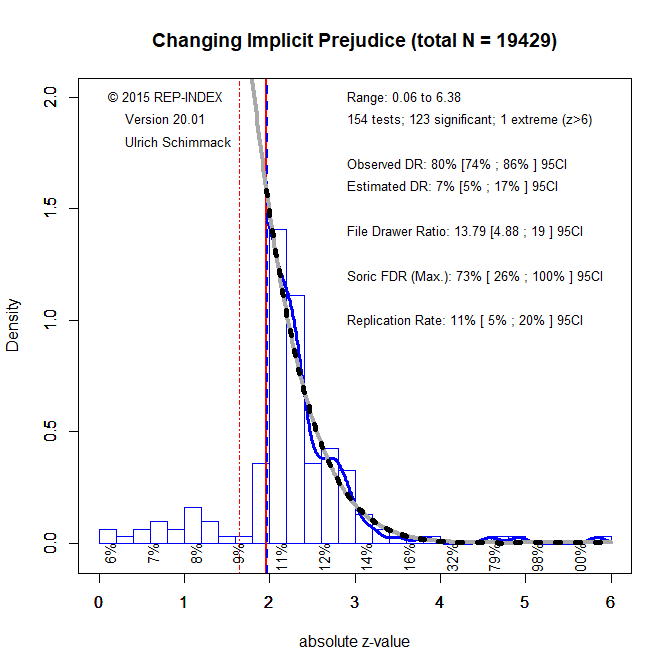
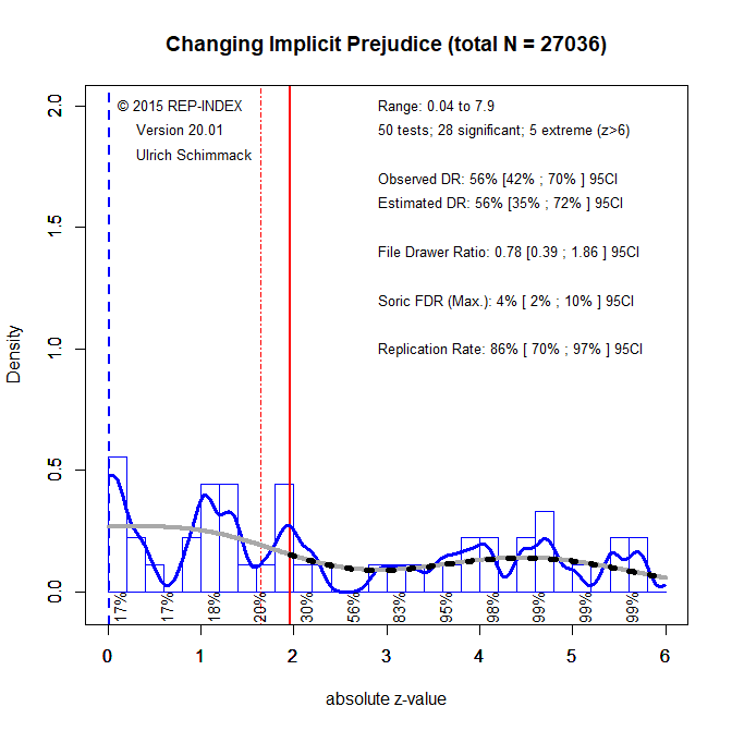
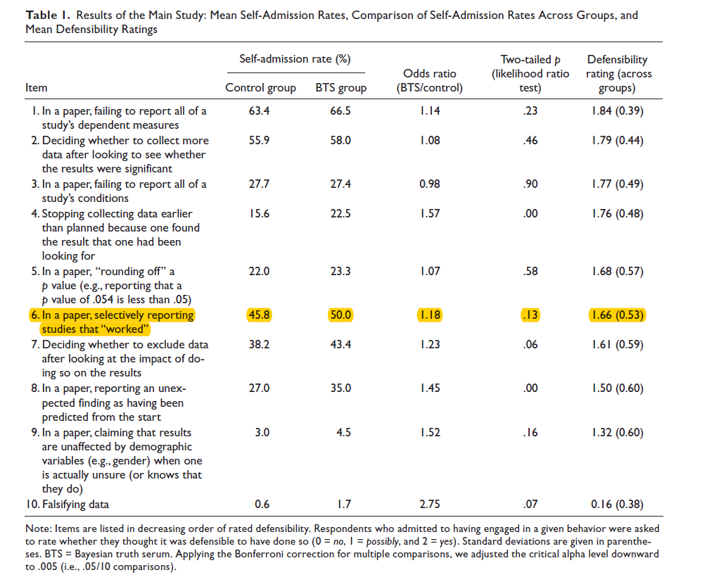
So far Simmons, Nelson, and Simonsohn have not commented on this blog post. I now submitted it as a commentary to JEP-General. Let’s see whether it will be send out for review and whether they will comment as (anonymous) reviewers.
Abstract
P-Curve was a first attempt to take the problem of selection for significance seriously and to evaluate whether a set of studies provides credible evidence against the null-hypothesis after taking selection bias into account. Here I showed that p-curve has serious limitations and provides misleading evidence about the strength of evidence against the null-hypothesis. I showed that all of the information that is provided by a p-curve analysis (Simonsohn, Nelson, & Simmons, 2014) is also provided by a z-curve analysis (Bartos & Schimmack, 2021). Moreover, z-curve provides additional information about the presence and the amount of selection bias. As z-curve is superior than p-curve, the rational choice is to use z-curve to examine the credibility of significant results.
Keywords: Publication Bias, Selection Bias, Z-Curve, P-Curve, Expected Replication Rate, Expected Discovery Rate, File-Drawer, Power
Introduction
In 2011, it dawned on psychologists that something was wrong with their science. Daryl Bem had just published an article with nine studies that showed an incredible finding (Bem, 2011). Participants’ responses were influenced by random events that had not yet occurred. Since then, the flaws in research practices have become clear and it has been shown that they are not limited to mental time travel (Schimmack, 2020). For decades, psychologists assumed that statistically significant results reveal true effects and reported only statistically significant results (Motyl et al., 2017; Sterling, 1959; Sterling et al., 1995). However, selective reporting of significant results undermines the purpose of significance testing to distinguish true and false hypotheses. If only significant results are reported, most published results could be false positive results (Simmons, Nelson, & Simonsohn, 2011).
Selective reporting of significant results also undermines the credibility of meta-analyses (Rosenthal, 1979), which explains why meta-analyses also suggest humans posses psychic abilities (Bem & Honorton, 1994). Thus, selection bias not only invalidates the results of original studies, it also threatens the validity of conclusions based on meta-analyses that do not take selection bias into account.
Concerns about a replication crisis in psychology led to an increased focus on replication studies. An ambitious project found that only 37% of studies in (cognitive & social) experimental psychology could be replicated (Open Science Collaboration, 2015). This dismal result created a crisis of confidence in published results. To alleviate these concerns, psychologists developed new methods to detect publication bias. These new methods showed that Bem’s paranormal results were obtained with the help of questionable research practices (Francis, 2012; Schimmack, 2012), which explained why replication attempts were unsuccessful (Galak et al., 2012). Furthermore, Francis showed that many published articles in the prestigious journal Psychological Science show signs of publication bias (Francis, 2014). However, the presence of publication bias does not imply that the published results are false (positives). Publication bias may merely inflate effect sizes without invalidating the main theoretical claims. To address the latter question it is necessary to conduct meta-analyses that take publication bias into account. In this article, I compare two methods that were developed for this purpose; p-curve (Simonsohn et al., 2014), and z-curve (Bartos & Schimmack, 2021; Brunner & Schimmack, 2020). P-curve was introduced in 2014 and has already been used in many articles. Z-curve was developed in 2015, but was only published recently in a peer-reviewed journal. Experimental psychologists who are familiar with speed-accuracy tradeoffs may not be surprised to learn that z-curve is a superior method. As Brunner and Schimmack (2020) demonstrated with simulation studies, p-curve often produces inflated estimates of the evidential value of original studies. This bias was not detected by the developers of p-curve because they did not evaluate their method with simulation studies. Moreover, their latest version of p-curve was never peer-reviewed. In this article, I first provide a critical review of p-curve and then show how z-curve addresses all of them.
P-Curve
P-curve is a name for a family of statistical tests that have been combined into the p-curve app that researchers can use to conduct p-curve analyses, henceforth called p-curve . The latest version of p-curve is version 4.06 that was last updated on November 30, 2017 (p-curve.com).
The first part of a p-curve analysis is a p-curve plot. A p-curve plot is a histogram of all significant p-values where p-values are placed into five bins, namely p-values ranging from 0 to .01, .01 to .02, .02 to .03, .03 to .04, and .04 to .05. If the set of studies contains mostly studies with true effects that have been tested with moderate to high power, there are more p-values between 0 and .01 than between .04 and .05. This pattern has been called a right-skewed distribution by the p-curve authors. If the distribution is flat or reversed (more p-values between .04 and .05 than between 0 and .01), the data lack evidential value; that is, the results are more consistent with the null-hypothesis than with the presence of a real effect.
The main limitation of p-curve plots is that it is difficult to evaluate ambiguous cases. To aid in the interpretation of p-curve plots, p-curve also provides statistical tests of evidential value. One test is a significance tests against the null-hypothesis that all significant p-values are false positive results. If this null-hypothesis can be rejected with the traditional alpha criterion of .05, it is possible to conclude that at least some of the significant results are not false positives. The main problem with this significance test is that it does not provide information about effect sizes. A right-skewed p-curve with a significant p-values may be due to weak evidence with many false positive results or strong evidence with few false positives.
To address this concern, the p-curve app also provides an estimate of statistical power. When studies are heterogeneous (i.e., different sample sizes or effect sizes or both) this estimate is an estimate of mean unconditional power (Bartos & Schimmack, 2021; Brunner & Schimmack, 2020). Unconditional power refers to the fact that a significant result may be a false positive result. Unconditional power does not condition on the presence of an effect (i.e., the null-hypothesis is false). When the null-hypothesis is true, a result has a probability of alpha (typically 5%) to be significant. Thus, a p-curve analysis that includes some false positive results, includes some studies with a probability equal to alpha and others with probabilities greater than alpha.
To illustrate the p-curve app, I conducted a meta-analysis of all published articles by Leif D. Nelson, one of the co-authors of p-curve I found 119 studies with codable data and coded the most focal hypothesis for each of these studies. I then submitted the data to the online p-curve app. Figure 1 shows the output.

Visual inspection of the p-curve plot shows a right-skewed distribution with 57% of the p-values between 0 and .01 and only 6% of p-values between .04 and .05. The statistical tests against the null-hypothesis that all of the significant p-values are false positives is highly significant. Thus, at least some of the p-values are likely to be true positives. Finally, the power estimate is very high, 97%, with a tight confidence interval ranging from 96% to 98%. Somewhat redundant with this information, the p-curve app also provides a significance test for the hypothesis that power is less than 33%. This test is not significant, which is not surprising given the estimated power of 97%.
The p-curve results are surprising. After all, Nelson openly stated that he used questionable research practices before he became aware of the high false positive risk associated with these practices. “We knew many researchers—including ourselves—who readily admitted to dropping dependent variables, conditions, or participants to achieve significance.” (Simmons, Nelson, & Simonsohn, 2018, p. 255). The impressive estimate of 97% power is in stark contrast to the claim that questionable research practices were used to produce Nelson’s results. A z-curve analysis of the data shows that the p-curve results provide false information about the robustness of Nelson’s published results.
Z-Curve
Like p-curve, z-curve analyses are supplemented by a plot of the data. The main difference is that p-values are converted into z-scores using the formula for the inverse normal distribution; z = qnorm(1-p/2). The second difference is that significant and non-significant p-values are plotted. The third difference is that z-curve plots have a much finer resolution than p-curve plots. Whereas p-curve bins all z-scores from 2.58 to infinity into one bin (p < .01), z-curve uses the information about the distribution of z-scores all the way up to z = 6 (p = .000000002; 1/500,000,000). Z-statistics greater than 6 are assigned a power of 1.

Visual inspection of the z-curve plot reveals something that the p-curve plot does not show, namely there is clear evidence for the presence of selection bias. Whereas p-curve suggests that “highly” significant results (0 to .01) are much more common than “just” significant results (.04 to .05), z-curve shows that just significant results (.05 to .005) are much more frequent than highly significant (p < .005) results. The difference is due to the implicit definition of high and low in the two plots. The high frequency of highly significant (p < .01) results in the p-curve plots is due to the wide range of values that are lumped together into this bin. Once it is clear that many p-values are clustered just below .05 (z > 1.96, the vertical red line), it is immediately notable that there are too few just non-significant (z < 1.96) values. This steep drop in frequencies for just significant to just not significant values is inconsistent with random sampling error. Thus, publication bias is readily visible by visual inspection of a z-curve plot. In contrast, p-curve plots provide no information about publication bias because non-significant results are not shown. Even worse, right skewed distributions are often falsely interpreted as evidence that there is no publication bias or use of questionable research practices (e.g., Rusz, Le Pelley, Kompier, Mait, & Bijleveld, 2020). This misinterpretation of p-curve plots can be easily avoided by inspection of z-curve plots.
The second part of a z-curve analysis uses a finite mixture model to estimate two statistical parameters of the data. These parameters are called the expected discovery rate and the expected replication rate (Bartos & Schimmack, 2021). Another term for these parameters is mean power before selection and mean power after selection for significance (Brunner & Schimmack, 2020). The meaning of these terms is best understood with a simple example where a researcher tests 100 false hypotheses and 100 true hypotheses with 100% power. The outcome of this study produces significant and non-significant p-values. The expected value for the frequency of significant p-values is 100 for the 100 true hypotheses tested with 100% power and 5% for the 100 false hypotheses that produce 5 significant results when alpha is set to 5%. Thus, we are expecting 105 significant results and 95 non-significant results. In this example, the discovery rate is 105/200 = 52.5%. With real data, the discovery rate is often not known because not all statistical tests are published. When selection for significance is present, the observed discovery rate is an inflated estimate of the actual discovery rate. For example, if 50 of the 95 non-significant results are missing, the observed discovery rate is 105/150 = 70%. Z-curve.2.0 uses the distribution of the significant z-scores to estimate the discovery rate by taking selection bias into account. That is, it uses the truncated distribution for z-scores greater than 1.96 to estimate the shape of the full distribution (i.e., the grey curve in Figure 2). This produces an estimate of the mean power before selection for significance. As significance is determined by power and sampling error, the estimate of mean power provides an estimate of the expected discovery rate. Figure 2 shows an observed discovery rate of 87%. This is in line with estimates of discovery rates around 90% in psychology journals (Motyl et al., 2017; Sterling, 1959; Sterling et al., 1995). However, the z-curve estimate of the expected discovery rate is only 27%. The bootstrapped, robust confidence interval around this estimate ranges from 5% to 51%. As this interval does not include the value for the observed discovery rate, the results provide statistically significant evidence that questionable research practices were used to produce 89% significant results. Moreover, the difference between the observed and expected discovery rate is large. This finding is consistent with Nelson’s admission that many questionable research practices were used to achieve significant results (Simmons et al., 2018). In contrast, p-curve provides no information about the presence or amount of selection bias.
The power estimate provided by the p-curve app is the mean power of studies with a significant result. Mean power for these studies is equal or greater to the mean power of all studies because studies with higher power are more likely to produce a significant result (Brunner & Schimmack, 2020). Bartos and Schimmack (2021) refer to mean power after selection for significance as the expected replication rate. To explain this term, it is instructive to see how selection for significance influences mean power in the example with 100 test of true null-hypotheses and 100 tests of true alternative hypotheses with 100% power. We expect only 5 false positive results and 100 true positive results. The average power of these 105 studies is (5 * .05 + 100 * 1)/105 = 95.5%. This is much higher than the mean power before selection for significance which was based on 100 rather than just 5 tests of a true null-hypothesis. For Nelson’s data, p-curve produced an estimate of 97% power. Thus, p-curve predicts that 96% of replication attempts of Nelson’s published results would produce a significant result again. The z-curve estimate in Figure 2 shows that this is a dramatically inflated estimate of the expected replication rate. The z-curve estimate is only 52% with a robust 95% confidence interval ranging from 40% to 68%. Simulation studies show that z-curve estimates are close to the simulated values, whereas p-curve estimates are inflated when the studies are heterogeneous (Brunner & Schimmack, 2020). The p-curve authors have been aware of this bias in p-curve estimates since January 2018 (Simmons, Nelson, & Simonsohn, 2018), but they have not changed their app or warned users about this problem. The present example clearly shows that p-curve estimates can be highly misleading and that it is unscientific to use or interpret p-curve estimates of the expected replication rate.
Published Example
Since p-curve was introduced, it has been cited in over 500 articles and it has been used in many meta-analyses. While some meta-analyses correctly interpreted p-curve results to demonstrate merely that a set of studies have some evidential value (i.e., the nil-hypothesis that all significant results are false positives), others went further and drew false conclusions from a p-curve analysis. Moreover, meta-analyses that used p-curve missed the opportunity to quantify the amount of selection bias in a literature. To illustrate how meta-analysts can benefit from a z-curve analysis, I reexamined a meta-analysis of the effects of reward stimuli on attention (Rusz, et al., 2020).

Using their open data (https://osf.io/rgeb6/), I first reproduced their p-curve analysis using the p-curve app (http://www.p-curve.com/app4/). Figure 3 show that 42% of the p-values are between .01 and 0, whereas only 7% of the p-values are between .04 and .05. The figure also shows that the observed p-curve is similar to the p-curve that is predicted by a homogeneous set of studies with 33% power. Nevertheless, power is estimated to be 52%. Rusz et al. (2020) interpret these results as evidence that “this set of studies contains evidential value for reward-driven distraction” and that “It provides no evidence for p-hacking” (p. 886).

Figure 4 shows the z-curve for the same data. Visual inspection of the z-curve plot shows that there are many more just-significant than just-not-significant results. This impression is confirmed by a comparison of the observed discovery rate (74%) versus the expected discovery rate (27%). The bootstrapped, robust 95% confidence interval, 8% to 58%, does not include the observed discovery rate. Thus, there is statistically significant evidence that questionable research practices inflated the percentage of significant results. The expected replication rate is also lower (37%) than the p-curve estimate (52%). With an average power of 37%, it is clear that published studies are underpowered. Based on these results, it is clear that effect-size meta-analysis that do not take selection bias into account produce inflated effect size estimates. Moreover, when the ERR is higher than the EDR, studies are heterogenous, which means that some studies have even less power than the average power of 37%, and some of these may be false positive results. It is therefore unclear which reward stimuli and which attention paradigms show a theoretically significant effect and which do not. However, meta-analysts often falsely generalize an average effect to individual studies. For example, Rusz et al. (2020) concluded from their significant average effect size (d ~ .3) that high-reward stimuli impair cognitive performance “across different paradigms and across different reward cues” (p. 887). This conclusion is incorrect because they mean effect size is inflated and could be based on subsets of reward stimuli and paradigms. To demonstrate that a specific reward stimulus influences performance on a specific task would require high powered replication studies for the various combinations of rewards and paradigms. At present, the meta-analysis merely shows that some rewards can interfere with some tasks.
Conclusion
Simonsohn et al. (2014) introduced p-curve as a statistical tool to correct for publication bias and questionable research practices in meta-analyses. In this article, I critically reviewed p-curve and showed several limitations and biases in p-curve results. The first p-curve methods focussed on statistical significance and did not quantify the strength of evidence against the null-hypothesis that all significant results are false positives. This problem was solved by introducing a method that quantified strength of evidence as the mean unconditional power of studies with significant results. However, the estimation method was never validated with simulation studies. Independent simulation studies showed that p-curve systematically overestimates power when effect sizes or sample sizes are heterogeneous. In the present article, this bias inflated mean power for Nelson’s published results from 52% to 97%. This is not a small or negligible deviation. Rather, it shows that p-curve results can be extremely misleading. In an application to a published meta-analysis, the bias was less extreme, but still substantial, 37% vs. 52%, a 15 percentage points difference. As the amount of bias is unknown unless p-curve results are compared to z-curve results, researchers can simply use z-curve to obtain an estimate of mean power after selection for significance or the expected replication rate.
Z-curve not only provides a better estimate of the expected replication rate. It also provides an estimate of the expected discovery rate; that is the percentage of results that are significant if all studies were available (i.e., after researchers empty their file drawer). This estimate can be compared to the observed discovery rate to examine whether selection bias is present and how large it is. In contrast, p-curve provides no information about the presence of selection bias and the use of questionable research practices.
In sum, z-curve does everything that p-curve does better and it provides additional information. As z-curve is better than p-curve on all features, the rational choice is to use z-curve in future meta-analyses and to reexamine published p-curve analyses with z-curve. To do so, researchers can use the free R-package zcurve (Bartos & Schimmack, 2020).
References
Bartoš, F., & Schimmack, U. (2020). “zcurve: An R Package for Fitting Z-curves.” R package version 1.0.0
Bartoš, F., & Schimmack, U. (2021). Z-curve.2.0: Estimating the replication and discovery rates. Meta-Psychology, in press.
Bem, D. J. (2011). Feeling the future: Experimental evidence for anomalous retroactive influences on cognition and affect. Journal of Personality and Social Psychology, 100, 407–425. http://dx.doi.org/10.1037/a0021524
Bem, D. J., & Honorton, C. (1994). Does psi exist? Replicable evidence for an anomalous process of information transfer. Psychological Bulletin, 115(1), 4–18. https://doi.org/10.1037/0033-2909.115.1.4
Brunner, J. & Schimmack, U. (2020). Estimating population mean power under conditions of heterogeneity and selection for significance. Meta-Psychology, 4, https://doi.org/10.15626/MP.2018.874
Francis, G. (2012). Too good to be true: Publication bias in two prominent studies from experimental psychology. Psychonomic Bulletin & Review, 19, 151–156. http://dx.doi.org/10.3758/s13423-012-0227-9
Francis G., (2014). The frequency of excess success for articles in Psychological Science. Psychonomic Bulletin and Review, 21, 1180–1187. https://doi.org/10.3758/s13423-014-0601-x
Galak, J., LeBoeuf, R. A., Nelson, L. D., & Simmons, J. P. (2012). Correcting the past: Failures to replicate. Journal of Personality and Social Psychology, 103, 933–948. http://dx.doi.org/10.1037/a0029709
Motyl, M., Demos, A. P., Carsel, T. S., Hanson, B. E., Melton, Z. J., Mueller, A. B., Prims, J. P., Sun, J., Washburn, A. N., Wong, K. M., Yantis, C., & Skitka, L. J. (2017). The state of social and personality science: Rotten to the core, not so bad, getting better, or getting worse? Journal of Personality and Social Psychology, 113(1), 34–58. https://doi.org/10.1037/pspa0000084
Open Science Collaboration. (2015). Estimating the reproducibility of psychological science. Science, 349(6251), aac4716–aac4716. https://doi.org/10.1126/science.aac4716
Rosenthal, R. (1979). The file drawer problem and tolerance for null results. Psychological Bulletin, 86(3), 638–641. https://doi.org/10.1037/0033-2909.86.3.638
Rusz, D., Le Pelley, M. E., Kompier, M. A. J., Mait, L., & Bijleveld, E. (2020). Reward-driven distraction: A meta-analysis. Psychological Bulletin, 146(10), 872–899. https://doi.org/10.1037/bul0000296
Schimmack, U. (2012). The ironic effect of significant results on the credibility of multiple-study articles. Psychological Methods, 17, 551–566. https://doi.org/10.1037/a0029487
Schimmack, U. (2020). A meta-psychological perspective on the decade of replication failures in social psychology. Canadian Psychology/Psychologie canadienne. 61 (4), 364-376. https://doi.org/10.1037/cap0000246
Simmons, J. P., Nelson, L. D., & Simonsohn, U. (2011). False-positive psychology: Undisclosed flexibility in data collection and analysis allows presenting anything as significant. Psychological Science, 22, 1359–1366. http://dx.doi.org/10.1177/0956797611417632
Simmons, J. P., Nelson, L. D., & Simonsohn, U. (2018). False-positive citations. Perspectives on Psychological Science, 13(2), 255–259. https://doi.org/10.1177/1745691617698146
Simonsohn, U., Nelson, L. D., & Simmons, J. P. (2014). P-curve: A key to the file-drawer. Journal of Experimental Psychology: General, 143(2), 534–547. https://doi.org/10.1037/a0033242
Sterling, T. D. (1959). Publication decision and the possible effects on inferences drawn from tests of significance – or vice versa. Journal of the American Statistical Association, 54, 30–34. https://doi.org/10.2307/2282137
Sterling, T. D., Rosenbaum, W. L., & Weinkam, J. J. (1995). Publication decisions revisited: The effect of the outcome of statistical tests on the decision to publish and vice versa. The American Statistician, 49, 108–112. https://doi.org/10.2307/2684823
