SUMMARY
In this blog post I show how it is possible to translate the results of a Bayesian Hypothesis Test into an equivalent frequentist statistical test that follows Neyman Pearsons approach of hypthesis testing where hypotheses are specified as ranges of effect sizes (critical regions) and observed effect sizes are used to make inferences about population effect sizes with long-run error rates.
INTRODUCTION
The blog post also explains why it is misleading to consider Bayes Factors that favor the null-hypothesis (d = 0) over an alternative hypothesis (e.g., Jeffrey’s prior) as evidence for the absence of an effect. This conclusion is only warranted with infinite sample sizes, but with finite sample sizes, especially small sample sizes that are typical in psychology, Bayes Factors in favor of H0 can only be interpreted as evidence that the population effect size is close to zero, but not as evidence that the population effect size is exactly zero. How close the effect sizes that are consistent with H0 are depends on sample size and the criterion value that is used to interpret the results of a study as sufficient evidence for H0.
Most researchers interpret Bayes Factors relative to some criterion value (e.g., BF > 3 or BF > 5 or BF > 10). These criterion values are just as arbitrary as the .05 criterion for p-values and the only justification for these values that I have seen is that (Jeffrey who invented Bayes Factors said so). There is nothing wrong with a conventional criterion value, even if Bayesian’s think there is something wrong with p < .05, but use BF > 3 in just the same way, but it is important to understand the implications of using a particular criterion value for an inference. In NHST the criterion value has a clear meaning. It means that in the long-run, the rate of false inferences (deciding in favor of H1 when H1 is false) will not be higher than the criterion value. With alpha = .05 as a conventional criterion, a research community decided that it is ok to have a maximum 5% error rate. Unlike, p-values, criterion values for Bayes-Factors provide no information about error rates. The best way to understand what a Bayes-Factor of 3 means is that we can assume that H0 and H1 are equally probable before we conduct a study and a Bayes Factor of 3 in favor of H0 makes it 3 times more likely that H0 is true than that H1 is true. If we were gambling on results and the truth were known, we would increase our winning odds from 50:50 to 75:25. With a Bayes-Factor of 5, the winning odds increase to 80:20.
HYPOTHESIS TESTING VERSUS EFFECT SIZE ESTIMATION
p-values and BF also share another shortcoming. Namely they provide information about the data given a hypothesis or two hypotheses, but they do not provide information about the data. We all know that we should not report results as “X influenced Y, p < .05”. The reason is that this statement provides no information about the effect size. The effect size could be tiny, d = 0.02, small, d = .20, or larger, d = .80. Thus, it is now required to provide some information about raw or standardized effect sizes and ideally also about the amount of raw or standardized sampling error. For example, standardized effect sizes could be reported as the standardized mean difference and sampling error (d = .3, se = .15) or as a confidence interval, e.g., (d = .3, 95% CI = 0 to .6). This is important information about the actual data, but it does not provide information about hypothesis tests. Thus, if the results of a study are used to test hypothesis, information about effect sizes and sampling errors has to be evaluated with specified criterion values that can be used to examine which hypothesis is consistent with an observed effect size.
RELATING HYPOTHESIS TESTS TO EFFECT SIZE ESTIMATION
In NHST, it is easy to see how p-values are related to effect size estimation. A confidence interval around the observed effect size is constructed by multiplying the amount of sampling error by a factor that is defined by alpha. The 95% confidence interval covers all values around the observed effect size, except the most extreme 5% values in the tails of the sampling distribution. It follows that any significance test that compares the observed effect size against a value outside the confidence interval will produce a p-value less than the error criterion.
It is not so straightforward to see how Bayes Factors relate to effect size estimates. Rouder et al. (2016) discuss a scenario where the 95% credibiltiy interval ranges around the most likey effect size of d = .165 ranges from .055 to .275 and excludes zero. Thus, an evaluation of the null-hypothesis, d = 0, in terms of a 95%CI would lead to the rejection of the point-zero hypothesis. We cannot conclude from this evidence that an effect is absent. Rather the most reasonable inference is that the population effect size is likely to be small, d ~ .2. In this scenario, Rouder et al. (2009) obtained a Bayes-Factor of 1. This Bayes-Factor also does not support H0, but it also does not provide support for H1. How is it possible that two Bayesian methods seem to produce contradictory results? One method rejects H0:d = 0 and the other method shows no more support for H1 than for H0:d = 0.
Rouder et al. provide no answer to this question. “Here we have a divergence. By using posterior credible intervals, we might reject the null, but by using Bayes’ rule directly we see that this rejection is made prematurely as there is no decrease in the plausibility of the zero point” (p. 536). Moreover, they suggest that Bayes Factors give the correct answer and the rejection of d = 0 by means of credibility intervals is unwarranted. “…, but by using Bayes’ rule directly we see that this rejection is made prematurely as there is no decrease in the plausibility of the zero point.Updating with Bayes’ rule directly is the correct approach because it describes appropriate conditioning of belief about the null point on all the information in the data” (p. 536).
The problem with this interpretation of the discrepancy is that Rouder et al. (2009) misinterpret the meaning of a Bayes Factor as if it can be directly interpreted as a test of the null-hypothesis, d = 0. However, in more thoughtful articles by the same authors, they recognize that (a) Bayes Factors only provide relative information about H0 in comparison to a specific alternative hypothesis H1, (b) the specification of H1 influences Bayes Factors, (c) alternative hypotheses that give a high a priori probability to large effect sizes favor H0 when the observed effect size is small, and (d) it is always possible to specify an alternative hypothesis (H1) that will not favor H0 by limiting the range of effect sizes to small effect sizes. For example, even with a small observed effect size of d = .165, it is possible to provide strong support for H1 and reject H0, if H1 is specified as Cauchy(0,0.1) and the sample size is sufficiently large to test H0 against H1.
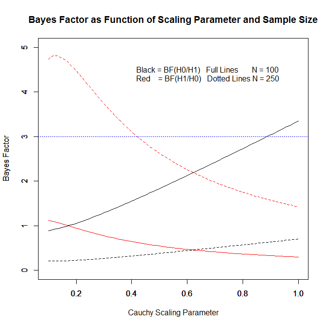
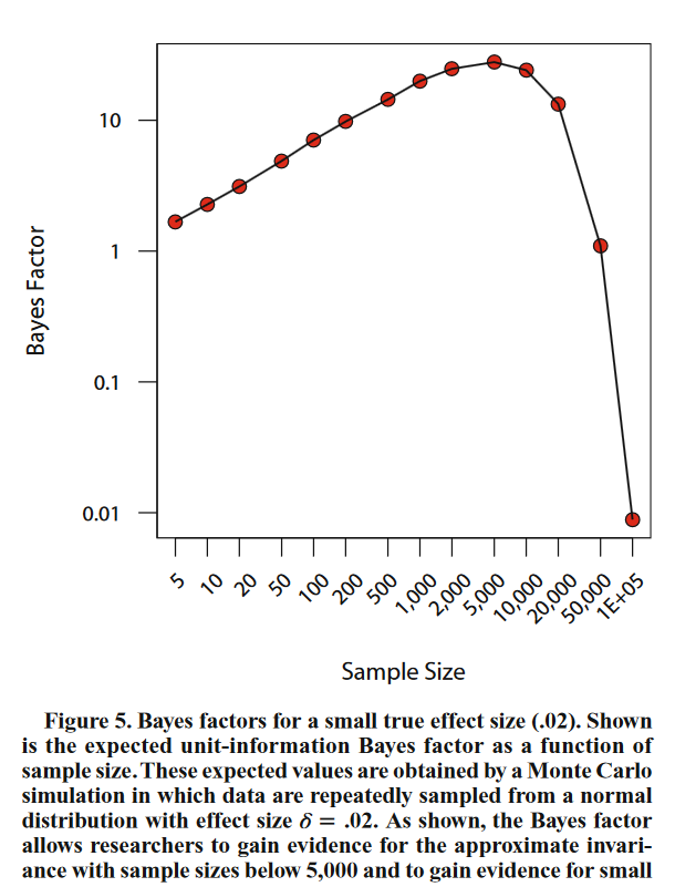
Figure 1 shows how Bayes Factors vary as a function of the specification of H1 and as a function of sample size with the same observed effect size of d = .165. It is possible to get Bayes-Factors greater than 3 in favor of H0 with a wide Cauchy (0,1) and a small sample size of N = 100 and a Bayes Factor greater than 3 in favor of H1 with a small scaling factor of .4 or smaller and a sample size of N = 250. In short, it is not possible to interpret Bayes Factors that favor H0 as evidence for the absence of an effect. The Bayes Factor only tells us that the observed effect size is more consistent with the data than H1, but it is difficult to interpret this result because H1 is not a clearly specified alternative effect size. H1 changes not only with the specification of the range of effect sizes, but also with sample size. This property is not a design flaw of Bayes Factors. They were designed to provide more and more stringent tests of H0:d = 0 that would eventually support H1 if the sample size is sufficiently large and H0:d = 0 is false. However, if H0 is false and H1 includes many large effect sizes (an ultrawide prior), Bayes Factors will first favor H0 and data collection may stop before Bayes Factors switch and provide the correct result that the population effect size is not zero. This behavior of Bayes-Factors was illustrated by Rouder et al. (2009) with a simulation of a population effect size of d = .02.
TRANSLATING RESULTS FROM A BAYESIAN HYPOTHESIS TEST INTO RESULTS FROM A NEYMAN PEARSON HYPOTHESIS TEST
The main effect of using Cauchy(0,1) to specify H1 is that the border value that distinguishes H0 and H1 is higher. The main effect of using BF.crit = 3 as a criterion value is that it is easier to provide evidence for H0 or H1 at the expense of having a higher error rate.
It is now possible to provide evidence for H0 with a small sample of n = 25 in a one-sample t-test. However, when we translate this finding into ranges of effect sizes, we see that the boundary between H0 and H1 is d = .39. Any observed effect size below .256 yields a BF in favor of H0. So, it would be misleading to interpret this finding as if a BF of 3 in a sample of n = 25 provides evidence for the point null-hypothesis d = 0. It only shows that an effect size of d < .39 is more consistent with an effect size of 0 than with effect sizes specified in H1 which places a lot of weight on large effect sizes. As sample sizes increase, the meaning of BF > 3 in favor of H0 changes. With N = 1,000, a BF of 3 any effect size larger than .071 does no longer provide evidence for H0. In the limit with an infinite sample size, only d = 0 would provide evidence for H0 and we can infer that H0 is true. However, BF > 3 in finite sample sizes does not justify this inference.
The translation of BF results into hypotheses about effect size regions makes it clear why BF results in small samples often seem to diverge from hypothesis tests with confidence intervals or credibility intervals. In small samples, BF are sensitive to specification of H1 and even if it is unlikely that the population effect size is 0 (0 is outside the confidence or credibility interval), the BF may show support for H0 because the effect size is below the criterion value that is needed to support H0. This inconsistency does not mean that different statistical procedures lead to different inferences. It only means that BF > 3 in favor of H0 RELATIVE TO H1 cannot be interpreted as a test of the hypothesis of d = 0. It can only be interpreted as evidence for H0 relative to H1 and the specification of H1 influences which effect sizes provide support for H0.
CONCLUSION
Sir Arthur Eddington (cited by Cacioppo & Berntson, 1994) described a hypothetical
scientist who sought to determine the size of the various fish in the sea. The scientist began by weaving a 2-in. mesh net and setting sail across the seas. repeatedly sampling catches and carefully measuring. recording. and analyzing the results of each catch. After extensive sampling. the scientist concluded that there were no fish smaller than 2 in. in the sea.
The moral of this story is that a scientists method influences their results. Scientists who use p-values to search for significant results in small samples, will rarely discover small effects and may start to believe that most effects are large. Similarly, scientists who use Bayes-Factors with wide priors may delude themselves that they are searching for small and large effects and falsely believe that effects are either absent or large. In both cases, scientists make the same mistake. A small sample is like a net with large holes that can only (reliably) capture big fish. This is ok, if the goal is to capture only big fish, but it is a problem when the goal is to find out whether a pond contains any fish at all. A wide net with big holes may never lead to the discovery of a fish in the pond, while there are plenty of small fish in the pond.
Researchers therefore have to be careful when they interpret a Bayes Factor and they should not interpret Bayes-Factors in favor of H0 as evidence for the absence of an effect. This fallacy is just as problematic as the fallacy to interpret a p-value above alpha (p > .05) as evidence for the absence of an effect. Most researchers are aware that non-significant results do not justify the inference that the population effect size is zero. It may be news to some that a Bayes Factor in favor of H0 suffers from the same problem. A Bayes-Factor in favor of H0 is better considered a finding that rejects the specific alternative hypothesis that was pitted against d = 0. Falsification of this specific H1 does not justify the inference that H0:d = 0 is true. Another model that was not tested could still fit the data better than H0.