The code for all simulations is available on OSF (https://osf.io/pyhmr).

P.S. I have been arguing with Andrew Gelman on his blog about his confusing and misleading article with Loken. Things have escalated and I just want to share his latest response.

Andrew on November 22, 2023 11:22 AM at 11:22 am said:

Ulrich:
I’m not dragging McShane into anything. You’re the one who showed up in the comment thread, mischaracterized his paper in two different ways, and called him an “asshole” for doing something that he didn’t do. You say now that you don’t care that he cited you; earlier you called him an asshole for not citing you, even though you did.

Also, your summaries of the McShane et al. and Gelman and Loken papers are inaccurate, as are your comments about confidence intervals, as are a few zillion other things you’ve been saying in this thread.

Please just stop it with the comments here. You’re spreading false statements and wasting our time; also I don’t think this is doing you any good either. I don’t really mind the insults if you had anything useful to say (here’s an example of where I received some critical feedback that was kinda rude but still very helpful), but whatever useful you have to say, you’ve already said, and at this point you’re just going around in circles. So, no more.

The main reason to share this is that I already showed that confidence intervals are often accurate even after selection for significance and that this is even more true when studies use unreliable measures because the attenuation due to random measurement error compensates for the inflation due to selection for significance. i am not saying that this makes it ok to suppress non-significant results, but it does show that Gelman is not interested in telling researchers how to avoid misinterpretation of biased point estimates. He likes to point out mistake in other people’s work, but he is not very good at noticing mistakes in his own work. I have repeatedly asked for feedback on my simulation results and if there are mistakes I am going to correct them. Gelman hasn’t done so and so far nobody else has. Of course, I cannot find a mistake in my own simulations. Ergo, I maintain that confidence intervals are useful to avoid misinterpretation of pointless point estimates. The real reason why confidence intervals are rarely interpreted (other than saying CI = .01 to 1.00 excludes zero, therefore the nil-hypothesis can be rejected, which is just silly nil-hypothesis testing, Cohen, 1994) is that confidence intervals in between-study designs with small samples are so wide that they do not allow strong conclusions about population effect sizes.

Introduction

A few years ago, Loken and Gelman (2017) published an article in the Magazine “Science.” A key novel claim in this article was that random measurement error can inflate effect size estimates.

“In a low-noise setting, the theoretical results of Hausman and others correctly show that measurement error will attenuate coefficient estimates. But we can demonstrate with a simple exercise that the opposite occurs in the presence of high noise and selection on statistical significance”

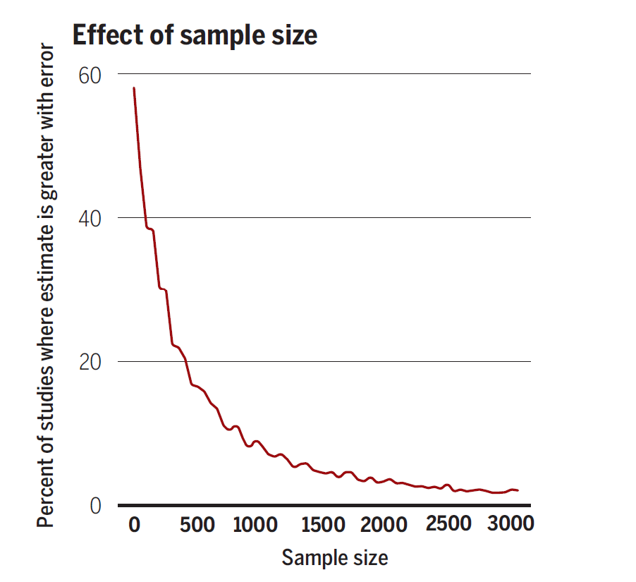
Language is famously ambiguous and open to interpretation. However, the article also presented a figure that seemed to support this counterintuitive conclusion.

–

The figure seems to suggest that with selection for significance, overestimation of effect sizes is increasingly more common in studies that use an unreliable measure rather than a reliable measure. At some point, the proportion of studies where the effect size estimate is greater with rather than without error seems to be over 50%.

Paradox findings are interesting and attracted our attention (Schimmack & Carlson, 2017). We believed that this conclusion is based on a mistake in the simulation code. We also tried to explain the combined effects of sampling error and random measurement error on effect sizes in a short commentary that remind unpublished. We never published our extensive simulation results.

Recently, a Ph.D student also questioned the simulation code and Andrew Gelman posted the students concerns on his blog post (Simulations of measurement error and the replication crisis: Maybe Loken and I have a mistake in our paper?) The blog post also included the simulation code.

The simulation is simple. It generates two variables with SD = 1 and a correlation ~ r = .15. It then adds 25% random measurement error to both variables, so that the two variables are measures of the former variables with 4/5 = 80% reliability. This attenuates the true correlation slightly to .15*.8 = .12. The crucial condition is when this simulation is run with a small sample size of N = 50.

N= 50 is a small sample size to study an effect size of .15 or .12. So, we are expecting mostly non-significant results. The crucial question is what happens when researchers get lucky and obtain a statistically significant result. Would selection for significance produce a stronger effect size estimate for the perfect measure or the unreliable measure?

It is not easy to answer this question because selection for significance requires conditioning on an outcome and Loken and Gelman’s simulation has two outcomes in the simulation. The outcomes for the perfect measure are paired with the outcome for the unreliable measure. So, which outcome should be used to select for significance? Using either measure will of course benefit the measure that was used to select for significance. To avoid this problem, I simply examined all four possible outcomes, neither measure was significant, the perfect measure was significant and the unreliable was not, the unreliable was significant and the perfect was not, or both were significant. To obtain stable cell frequencies, I ran 10,000 simulations.

Here are the results.

1. Neither measure produced a significant result

4870 times the perfect measure had a higher estimate than the unreliable measure (58%)
3629 times the unreliable measure had a higher estimate than the unreliable measure (42%)

2. Both measure produced a significant result

579 times the perfect measure had a higher estimate than the unreliable measure (61%)
377 times the unreliable measure had a higher estimate than the unreliable measure (39%)

3. The reliable measure is significant and the unreliable measure is not significant

981 times the perfect measure had a higher estimate than the unreliable measure (100%)
0 times the unreliable measure had a higher estimate than the unreliable measure (0%)

4. The unreliable measure is significant and the reliable measure is not significant

0 times the perfect measure had a higher estimate than the unreliable measure (0%)
464 times the unreliable measure had a higher estimate than the unreliable measure (100%)

The main point of these results is that selection for significance will always favor the measure that is used for conditioning on significance. By definition, the effect size of a significant result will be larger than the effect size of a non-significant result given equal sample size. However, it is also clear that the unreliable measure produces fewer significant results because random measurement error attenuates the effect size and reduces power; that is, the probability to obtain a significant result.

Based on these results, we can reproduce Loken and Gelman’s results that showed larger effect size estimates more often with the unreliable measure. To produce this result, they conditioned on significance for the measure with random error, but not for the measure without random measurement error. That is, they combined conditions 2 (both measures produced significant results) and 4 (ONLY the unreliable measure produced significant result).

5. (2 + 4) The unreliable measure is significant, the reliable measure can be significant or not significant.

When we simply select for significance on the unreliable measure, we see that the unreliable measure has the stronger effect size over 50% of the time.

579 times the perfect measure had a higher estimate than the unreliable measure (41%)
377+464 = 841 times the unreliable measure had a higher estimate than the unreliable measure (59%)

However, this is not a fair comparison of the two measures. Selection for significance is applied to one of them and not the other. The illusion of reversal is produced by selection bias in the simulation, not in a real world scenario where researchers use one or the other measure. This is easy to see, when we condition on the reliable measure.

6. (2 + 3) The reliable measure is significant, significance on the other measure does not matter.

579+981 = 1560 times the perfect measure had a higher estimate than the unreliable measure (81%)
377 times the unreliable measure had a higher estimate than the unreliable measure (19%)

Now, we overestimate the advantage of the reliable measure. Conditioning on significance selectively for one variable and not the other produces biased simulation results that falsely suggest that an unreliable measure produces stronger correlations despite the fact that random measurement error attenuates correlation coefficients and other standardized effect size estimates.

Extension 1: A Fair Comparison

I posted polls on Twitter (X) and in a Facebook Group that discusses methodological issues in psychological science. I created a scenario in which two labs are studying the same effect, say r = .15 in the population between two variables. Both labs use the same small sample size of N = 50. Both labs only publish when they get a statistically significant result, p < .05 (two-tailed). Both labs use a perfectly reliable preditor variable (e.g., height). The only difference between the two labs is that LAB A uses a more reliable measure (Cronbach’s alpha = .8) than LAB B (Cronbach’s alpha = .5). The question is simply which lab is more likely to publish a bigger (more biased) effect size estimate? The key difference between this scenario and Loken and Gelman’s simulation is that both outcomes are conditioned on significance. Thus, we can actually see the influence of random measurement error on correlation coefficients when results are selected for significance. The polls showed that the correct answer is unknown. In both polls, two-third of respondents sided with Loken and Gelman and answered that LAB B is more likely to report larger correlations (Twitter/X 65%, Facebook Group, 68%). They may have been influenced by Loken and Gelman’s article that claimed “in noisy research settings, poor measurement can contribute to exaggerated estimates of effect size.”

ChatGPT on Bing thinks LAB A will report stronger effect sizes, but its reasoning does not take conditioning for significance into account. “According to the results, the effect size is a measure of the magnitude of the experimental effect, and it is influenced by the reliability of the measures used. The higher the reliability, the more accurate the effect size estimate will be¹. Therefore, LAB A, which uses a more reliable measure (Cronbach’s alpha = .8) than LAB B (Cronbach’s alpha = .5), is more likely to publish a bigger (more biased) effect size estimate. LAB B, which uses a less reliable measure, will have more measurement error and lower statistical power, making it harder to detect the true effect size in the population.”

To obtain the correct answer, I made only a small change to Loken and Gelman’s simulation. First, I did not add measurement error to the predictor variable, X. Second, I added different amounts of random measurement error to two outcome variables, Y1 with 80% reliable variance for LAB A, and y2 with 50% reliable variance for LAB B. I ran 10,000 simulations to have a reasonably large number of cases after selection for significance. LAB A had more significant results because the population effect size or average sample correlation is larger, .15 * .8 = .12 than the one for LAB B, .15 * .5 = .075, and studies with larger effect sizes in the same sample size have more statistical power, a greater chance to produce a significant result. In the simulation, LAB A had 1,435 significant results (~ 14% power) and LAB B had 1,106 significant results (11% power). I then compared the first 1,106 significant results from LAB A to the 1,106 results from LAB B and computed how often LAB A had a higher effect size estimate than LAB B.

Results: LAB A had a higher effect size estimate in 569 cases (51%) and LAB B had a higher effect size estimate in 537 cases (49%). Thus, there is no reversal that less reliable measures produce stronger (more biased) correlations in studies with low power and after selection for significance. Loken and Gelman’s false conclusion is based on an error in their simulations that conditioned on significance for the unreliable measure, but not for the measure without random measurement error.

Would a more extreme scenario produce a reversal? Power is already low and nobody should compute correlation coefficients in samples with N = 20, but fMRI researchers famously reported dramatic correlations between brain and behavior i studies with N = 8 (“voodoo correlations; Vul et al., 2012). So, I repeated the simulation with N = 20, and pitting a measure with 100% reliability against a measure with 20% reliability. Given the low power, I ran 100,000 simulations to get stable results.

Results:

LAB A obtained 9,620 significant results (Power ~ 10%). LAB B obtained 6,030 (Power ~ 6%, close to chance, 5% with alpha = .05).

The comparison of the first 6,030 significant results with the 6,030 significant results from LAB B showed that LAB A reported a stronger effect size 3,227 times (54%) and LAB B reported a stronger effect size 2,803 times (46%). Thus, more reliable not only help to report voodoo correlations more often, but also report higher correlations. Clearly, using less reliable measures does not contribute to the replication crisis as Loken and Gelman claimed. Their claim is based on a mistake in their simulations that conditioned joked outcomes on significance of the unreliable measure.

Extension 2: Simulation with two equally unreliable measures

The next simulation is a new simulation that has two purposes. First, it drives home the message that Gelman’s simulation study unfairly biased the results in favor of the unreliable measure by conditioning on significance for this measure. Second, it provides a new insight into the contribution of unreliable measures to the replication crisis. The simulation assumes that researchers really use two dependent variables (or more) and are going to report results if at least one of the measures has a significant result. Evidently, this doesn’t really work with two perfect measures because they are perfectly correlated, r = 1. As a result, they will always show the same correlation with the independent variable. However, unreliable measures are not perfectly correlated with each other and produce different correlations. This provides room for capitalizing on chance and getting significance with low power. The lower the reliability of the measures the better. I picked a reliability of .5 for both dependent measures (Y1, Y2) and assumed that the independent variable has perfect reliability (e.g., an experimental manipulation).

1. Neither measure produced a significant result

4011 times Y1 had a higher estimate than Y2 (49%)
4109 times Y2 had a higher estimate than Y1 (51%).

2. Both measures produced a significant result.

212 times Y1 had a higher estimate than Y2 (57%)
162 times Y2 had a higher estimate than Y1 (43%).

3. Y1 is significant and Y2 is not significant

743 times Y1 had a higher estimate than Y2 (100%)
0 times Y2 had a higher estimate than Y1 (0%).

4. Y2 is significant and Y1 is not significant

0 times Y1 had a higher estimate than Y2 (0%)
763 times Y2 had a higher estimate than Y1 (100%).

The results show that using two measures with 50% reliability increases the chances of obtaining a significant result by about 750 / 10000 tries (7.5 percentage points). Thus, unreliable measures can contribute to the replication crisis if researchers use multiple unreliable measures and selectively publish results for the significant one. However, using a single unreliable measure versus a single reliable measure is not beneficial because an unreliable measure makes it less likely to obtain a significant result. Gelman’s reversal is an artifact by conditioning on one outcome. This can be easily seen by comparing the results after conditioning on significance for Y1 or Y2.

5. (2 + 3) Y1 is significant, significance of Y2 does not matter

212+743 = 955 times Y1 had a higher estimate than Y2 (85%)
162 times Y2 had a higher estimate than Y1 (15%).

6. (2 + 4) Y2 is significant, significance of Y1 does not matter

212 = times Y1 had a higher estimate than Y2 (81%)
162+763 = 925 times Y2 had a higher estimate than Y1 (19%).

When we condition on significance for Y1, Y1 produces more often significant results. When we condition on Y2, Y2 produces more often significant results. This has nothing to do with the reliability of the measures because they have the same reliability. The difference is illusory because selection for significance in the simulation produces biased results.

Another interesting observation

While working on this issue with Rickard, we also discovered an important distinction between standardized and unstandardized effect sizes. Loken and Gelman simulated standardized effect sizes because by correlating two variables. Random measurement error lowers standardized effect sizes because the unstandardized effect sizes are divided by the standard deviation and random measurement error adds to the naturally occurring variance in a variable. However, unstandardized effect sizes like the covariance or the mean difference between two groups are not attenuated by random measurement error. For this reason, it would be wrong to claim that unreliability of a measure attenuated unstandardized effect sizes or that they should be corrected for unreliability of a measure.

Random measurement error will however increase the standard error and make it more difficult to get a significant result. As a result, selection for significance will inflate the unstandardized effect size more for an unreliable measure. The following simulation demonstrates this point. To keep things similar, I kept the effect size of b = .15, but used the unstandardized effect size of a regression analysis as the effect size.

First, I show the distribution of the effect size estimates. Both distributions are centered over the simulated effect size of b = .15. However, the measure with random error produces a wider distribution which often results in more extreme effect size estimates.

1. Neither measure produced a significant result

3170 times the perfect measure had a higher estimate than the unreliable measure (41%)
4587 times the unreliable measure had a higher estimate than the unreliable measure (59%)

This scenario shows the surprising reversal that the less reliable measure shows the stronger absolute effect size estimates more often and more than 50% of the time that Loken and Gelman wanted to demonstrated, but their simulation used standardized effect size estimates that do not produce this reversal. Only unstandardized effect size estimates show it.

2. Both measures produced a significant result

73 times the perfect measure had a higher estimate than the unreliable measure (10%)
659 times the unreliable measure had a higher estimate than the unreliable measure (90%)

When both effect size estimates are significant, the one with the unreliable measure is much more likely to show a stronger effect size estimate. The reason is simple. Sampling error is larger and it takes a stronger effect size estimate to produce the same t-value that produces a significant result.

3. The reliable measure is significant and the unreliable measure is not significant

790 times the perfect measure had a higher estimate than the unreliable measure (73%)
299 times the unreliable measure had a higher estimate than the unreliable measure (27%)

With standardized effect sizes, selection for significance always favored the conditioning variable 100% of the time. Now unstandardized coefficients are higher 27% of the time. However, the conditioning effect is notable because conditioning on significance for the perfect measure reverses the usual pattern that the unreliable measure produces stronger effect size estimates.

4. The unreliable measure is significant and the reliable measure is not significant

0 times the perfect measure had a higher estimate than the unreliable measure (0%)
422 times the unreliable measure had a higher estimate than the unreliable measure (100%)

Conditioning on significance on the unreliable measure produces a 100% rate of stronger effect sizes because effect sizes are already biased in favor of the unreliable measure.

The interesting observation is that Loken and Gelman were right that effect size estimates can be inflated with unreliable measures, but they failed to demonstrate this reversal because they used standardized effect size estimates. Inflation occurs with unstandardized effect sizes. Moreover, it does not require selection for significance. Even non-significant effect size estimates tend to be larger because there is more sampling error.

The Fallacy of Interpreting Point Estimates of Effect Sizes

Loken and Gelman’s article is framed as a warning to practitioners to avoid misinterpretation of effect size estimates. The are concerned that researchers “assume that the observed effect size would have been even larger if not for the burden of measurement error” and “when it comes to surprising research findings from small studies, measurement error (or other uncontrolled variation) should not be invoked automatically to suggest that effects are even larger” and “our concern is that researchers are sometimes tempted to use the “iron law” reasoning to defend or justify surprisingly large statistically significant effects from small studies”

They missed an opportunity to point out that there is a simple solution to avoid misinterpretation of effect sizes estimates that has been recommended by psychological methodologists since the 1990s (I highly recommend Cohen, 1994; also Cummings, 2013). The solution is to consider the uncertainty in effect sizes estimates by means of confidence intervals. Confidence provide a simple solution to many fallacies of traditional null-hypothesis tests, p < .05. A confidence interval can be used to test not only the nil-hypothesis, but also hypotheses about specific effect sizes. A confidence interval may exclude zero, but it might include other values of theoretical interest, especially if sampling error is large. To claim an effect size larger than the true population effect size of b = .15, the confidence interval has to exclude a value of b = .15. Otherwise, it is a fallacy to claim that the effect size in the population is larger than .15.

As demonstrated before, random measurement error inflates effect size estimates of unstandardized effect sizes, but it also increases sampling error, resulting in wider confidence interval. Thus, it is an important question whether unreliable measures really allow researchers to claim effect sizes that are significantly larger than the simulated true effect size of b = .15.

A final simulation examined how often the 95%CI excluded the true value of b = .15 for the perfect measure and the unreliable measure. To produce more precise estimates, I ran 100,000 simulations.

1. Measure without error

2809 Significant underestimations (2.8%)
2732 Significant overestimations (2.7%)
5541 Errors

2. Measure with error

2761 Significant underestimations (2.8%)
2750 Significant overestimations (2.7%)
5511 Errors

The results should not come as a surprise. 95% confidence intervals are designed to have a 5% error rate and to split these errors into equal errors on both sides. The addition of random measurement error does not affect this property of confidence intervals. Most important, there is no reversal in the probability of overestimation. The measure without error produces confidence intervals that overestimate the true effect size as often as the measure without error. However, the effect of random measurement error is noticeable in the amount of bias.

For the measure without error, the lower bound of the 95%CI ranges from .15 to .55, M = .21.
For the measure with error, the lower bound of the 95%CI ranges from .15 to .65, M = .22.

These differences are small and have no practical consequences. Thus, the use of confidence intervals provides a simple solution to false interpretation of effect size estimates. Although selection for significance in small samples inflates the point estimate of effect sizes, the confidence interval often includes the smaller true effect size.

The Replication Crisis

Loken and Gelman’s article aimed to relate random measurement error to the replication crisis. They write “If researchers focus on getting statistically significant estimates of small effects, using noisy measurements and small samples, then it is likely that the additional sources of variance are already making the t test look strong. Measurement error and selection bias thus can combine to exacerbate the replication crisis.”

The previous results show that this statement ignores the key influence of random measurement error on statistical significance. Random measurement error increases the standard deviation and the standard deviation is in the denominator of the t-statistic. Thus, t-values are biased downwards and it is harder to get statistical significance with unreliable measures. The key point is that studies in small samples with unreliable measures have low statistical power. It is therefore misleading to claim that random-measurement error inflates t-values. It actually attenuates t-values. Selection for significance inflates point estimates of effect sizes, but these are meaningless and the confidence interval around this estimate often include the true population parameter.

More important, it is not clear what Loken and Gelman mean by the replication crisis. Let’s assume a researcher conducts a study with N = 50, a measure with 50% reliability, and an effect size of r = .15. Luck, the winner’s curse, gives them a statistically significant result with an effect size estimate of r = .6 and a 95% confidence interval ranging from .42 to .86. They get a major publication out of this finding. Another researcher conducts a replication study and gets a non-significant result with r = .11 and a 95%CI ranging from -.11 to .33. This outcome is often called a replication failure because significant results are considered successes and non-significant results are considered failures. However, findings like this do not signal a crisis. Replication failures are normal and to be expected because significance testing allows for error and replication failures.

The replication crisis in psychology is caused by the selective omission of replication failures from the literature or even from a set of studies within a single article (Schimmack, 2012). The problem is not that a single significant result is followed by a non-significant result. The problem is that non-significant results are not published. The success rate in psychology journals is over 90% (Sterling, 1959; Sterling et al., 1995). Thus, the replication crisis refers to the fact that psychologists never published failed replication studies. When publication of replication failures became more acceptable in the past decade, we just saw that selection bias inflated the success rate. Given the typical power of studies in psychology, replication failures are to be expected. This has nothing to do with random measurement error. The main contribution of random measurement error is to reduce power and increase the percentage of studies with non-significant results.

Forgetting about False Negatives

Over the past decade, a few influential articles have created a fear of false positive results (Ioannidis, 2005; Simmons, Nelson, & Simonsohn, 2011). The real problem, however, is that selection for significance makes it impossible to know whether an effect exists or not. Whereas real effects in reasonably powered studies would often produce significant results, false positives would be followed by many replication failures. Without credible replication studies that are published independent of the outcome, statistical significance has no meaning. This led to concerns that over 50% of published results could be false positives. However, empirical studies of the false positive risk often find much lower plausible values (Bartos & Schimmack, 2023). Arguably, the bigger problem in studies with small samples and unreliable measures is that these studies will often produce a false negative result. Take, Loken and Gelman’s simulation as an example. The key outcome of studies that look for a small effect size of r = .15 or r = .12 with a noisy measure is a non-significant result. This is a false negative result because we know a priori that there is a non-zero correlation between the two variables with a theoretically important effect size. For example, the correlation between income and a noisy measure of happiness is around r = .15. Looking for this small relationship in a small sample will often suggest that money does not buy happiness, while large samples consistently show this small relationship. One might even argue that the few studies that produce a significant result with an inflated point estimate but a confidence interval that includes r = .15 avoid the false negative result without providing inflated estimates of the effect size given the wide range of plausible values. Only the 2.5% of studies that produce confidence intervals that do not include r = .15 are misleading, but a single replication study is likely to correct this inflated estimate.

This line of reasoning does not justify selective publishing of significant results. Rather it draws attention back to the concerns of methodologists in the 1990s that low power is wasteful because many studies produce inconclusive results. To address this problem researchers need to think carefully about the plausible range of effect sizes and plan studies that can produce significant results for real effects. Researchers also need to be able and willing to publish results when the results are not significant. No statistical method can produce valid results when the data are biased. In comparison, the problem of inflated point estimates of effect sizes in a single small sample is trivial. Confidence interval make it clear that the true effect size can be much smaller and rare outcomes of extreme inflation will be corrected quickly by failed replication studies.

In short, as much as Gelman likes to think that there is something fundamentally wrong with the statistical methods that psychologists use, the real problems are practical. Resource constraints often limit researchers ability to collect large samples and the preference for novel significant results over replication failures of old findings gives researchers an incentive to selectively report their “successes.” To do so, they may even use multiple unreliable measures in order to capitalize on chance. The best way to address these problems is to establish a clear code of research practices and to hold researchers accountable if they violate this code. Editors should also enforce the already existing guidelines to report meaningful effect sizes with confidence intervals. In this utopian world, researchers would benefit from using reliable measures because they increase power and the probability of publishing a true positive result.

Abandon Gelman

I pointed out the mistake in Loken and Gelman’s article on Gelman’s blog post. He is unable to see that his claim of a reversal in effect size estimates due to random measurement error is a mistake. Instead he tries to explain my vehement insistence as a personality flaw.

Instead, his overconfidence makes it impossible to consider the possibility that he made a mistake. This arrogant response to criticism is by no means unique. I have seen it many times by Greenwald, Bargh, Baumeister, and others. However, it is ironic when meta-scientists like Ioannidis, Gelman, or Simonsohn who are known for harsh criticism of others are unable to admit when they made a mistake. A notable exception is my criticism of Kahneman’s book “Thinking: Fast and Slow.”

Gelman has criticized psychologists without offering any advice how they could improve their credibility. His main advice is to “abandon statistical significance” without any guidelines how we should distinguish real findings from false positives or avoid interpretation of inflated effect size estimates. Here I showed how the use of confidence intervals provides a simple solution to avoid many of the problems that Gelman likes to point out. To learn about statistics, i suggest to read less Gelman and read more Cohen.

Cohen’s work shaped my understanding of methodology and statistics and he actually cared about psychology and tried to improve it. Without him, I might not have learned about statistical power or contemplated the silly practice of refuting nil-hypothesis. I also think his work was influential in changing the way results are reported in psychology journals that enabled me to detected biases and estimate false positive rates in our field. He also tried to tell psychologists about the importance of replication studies.

For generalization, psychologists must finally rely, as has been done in all the older sciences, on replication” (Cohen, 1994).

If psychologists had listened to Cohen, they could have avoided the replication crisis in the 2010s. However, his work can still help psychologists to learn from the replication crisis to build a credible science that is build on true positive results and avoids false negative results. The lessons are simple.
1. Plan studies with a reasonable chance to get a significant result. Try to maximize power by thinking about all possible ways to reduce sampling error, including using more reliable measures.
2. Publish studies independent of outcome, especially replication failures that can correct false positives.
3. Focus on effect sizes, but ignore the point estimates. Instead, use confidence interval to avoid interpreting effect size estimates that are inflated by selection for significance.