Mertens, S., Herberz, M., Hahnel, U. J. J., & Brosch, T. (2022). The effectiveness of nudging: A meta-analysis of choice architecture interventions across behavioral domains. Proceedings of the National Academy of Sciences, 119(1), e2107346118. https://doi.org/10.1073/pnas.2107346118

Introduction

Hundreds of studies examined the effectiveness of nudging manipulations, and most of them reported a positive effect, often also a statistically significant one; that is, a result unlikely to be a statistical fluke. A 2022 meta-analysis included 447 effect sizes from 212 publications. The pooled meta-analytic estimate was—not 42, but 43; that is d = .43 or 43% of a standard deviation.

This answer is close to the famous answer to the question about the meaning of life, the universe, and everything else in The Hitchhiker’s Guide to the Galaxy, which was 42. The novel poked fun at the attempt to answer a complex question with a single number, but meta-analyses often do exactly this. The hundreds of studies in the nudging literature used different manipulations, different outcomes, and different populations. What is the probability that they all have the same effect size? Nil. So, the headline figure in a meta-analysis is at best the center of a heterogeneous distribution of effect sizes; it does not tell us the effect of any specific intervention.

This did not stop two research teams from reanalyzing the data with statistical methods designed to correct for publication bias and to produce another single number. This number was dramatically different. Szászi et al. (2022) used a step-function selection model and obtained an adjusted estimate of the average effect size of $d=-.01$, with a very small standard error, $SE=.02$. In other words, after bias correction, the average effect of nudging was now approximately zero.

A second commentary reported the results of another analysis using a new statistical method, Robust Bayesian Meta-Analysis (RoBMA), which averages across several models, including one similar to the model used by Szászi et al. (2022). The title of the article—which is the only thing many readers ever see—made the conclusion clear: “No evidence for nudging after adjusting for publication bias” (Maier et al., 2022). Their estimated average effect size, $d=.04$, was not exactly zero, but close enough to invite the interpretation that nudging effects are negligible or nonexistent.

There are several problems with both reanalyses that presented the average estimate as the key finding. The first one is that the average alone is meaningless, when the same model also estimates considerable heterogeneity around the average. Neither article reported the estimate of heterogeneity that the models produce, but a reanalysis of the data with the models shows considerable heterogeneity (weight-function model, sd = .5; RoBMA sd = .3). This implies that many positive effect sizes estimates were obtained with positive population effect sizes that can be replicated. Thus, the results do not imply that nudging never has an effect. At least sometimes, nudging had effects. This simple fact is easily conveyed by a figure that plots the predicted distributions of population effect sizes along with the distribution of observed effect sizes (Figure 1).

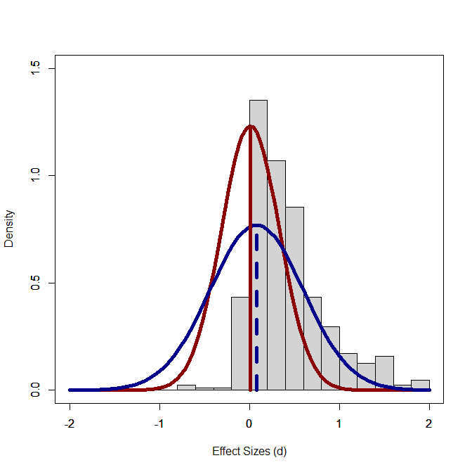
The histogram shows that 91% of the observed effect-size estimates are positive. In contrast, the fitted distributions of population effect sizes are centered close to zero and therefore imply nearly equal numbers of positive and negative true effects. How can models that imply so many negative effects fit data in which negative estimates are rare?

The answer lies in two assumptions built into the models. First, they assume that population effect sizes follow a normal distribution. The positive observed effects are concentrated near zero with a long right tail and therefore resemble the positive half of a normal distribution centered close to zero. Once the model places the center near zero, however, symmetry requires a corresponding negative half. Because this negative half is largely missing from the observed data, the discrepancy is attributed to selection: negative results are assumed to be observed, but remained unpublished.

But this is not the only explanation of the observed pattern. An alternative is that there really are relatively few negative population effects—that is, nudges usually have effects in the theoretically predicted direction—but that the distribution of positive effects is strongly non-normal. Most nudges may have effects close to zero, while a smaller number have moderate or large positive effects. Such a right-skewed distribution would also produce exactly what we see in the histogram: many small positive effects, relatively few negative effects, and a long positive tail.

The crucial point is that the models cannot distinguish these two explanations from the observed data alone. A symmetric distribution centered near zero combined with strong selection against negative results can resemble an asymmetric population distribution containing mostly positive effects and little or no selection against negative results. The near-zero mean therefore does not follow directly from the data. It follows from the assumption that the underlying distribution of population effects is approximately normal and symmetric.

Separating Positive and Negative Results

Fortunately, we do not have to decide which explanation is correct to learn something useful from these models. If all variation in observed effect sizes were merely sampling error around a single population effect, positive and negative estimates would have to be combined to estimate that common effect. But both models estimate substantial heterogeneity. In their own models, population effect sizes genuinely differ from one study to another.

We can therefore ask a different question. Rather than averaging positive and negative population effects into a single number, we can examine the two parts of the fitted distribution separately. In particular, we can ask: Among population effects that are in the theoretically predicted direction, what is their average magnitude? If desired, we could ask the corresponding question about effects in the opposite direction.

This is a different estimand from the grand mean. It is also important to distinguish it from simply averaging the 91% of observed estimates that are positive. Observed estimates contain sampling error, and some positive estimates may arise from population effects close to zero or even negative. Instead, we can use the models’ estimated normal distribution of population effect sizes to calculate the mean of the positive part of the normal distribution.

RoBMA’s estimate is d = .26, a small effect, but the step-function model produces an estimate of d = .44, very similar to the estimate of d = .43 in the original article that was based on all estimates. The mean of only positive results is d = .51, but it is reduced to d = .43 by the inclusion of the negative results.

In conclusion, the two critical reanalyses that reduced the estimated grand mean from about $d=.43$ to approximately zero did not show that the positive effects themselves were reduced to zero after correcting for publication bias. In the step-function model, the estimated mean of positive population effects remains $d=.44$. Even RoBMA implies an average positive population effect of $d=.26$. The dramatic change in the grand mean arises largely because the models infer a substantial population of unobserved negative effects that counterbalances the positive effects.

Those missing negative effects may exist. Researchers may have obtained effects in the theoretically wrong direction and failed to publish them. But this does not imply that the positive effects are zero, nor does it show that their magnitudes were dramatically inflated. In particular, the step-function model provides little evidence that selection for statistical significance—the usual mechanism invoked to explain inflated published effect sizes—accounts for the observed pattern. Its strongest selection effect is for the direction of the effect: negative results are much less likely to appear.

This makes the presentation of the reanalyses misleading. The headline result was the grand mean close to zero, while the substantial heterogeneity around that mean was not reported in a way that made clear that the model implied a broad distribution of positive and negative effects. Nor was the weak evidence for selection at the conventional significance threshold emphasized. A very different headline could therefore have been: “Little evidence that selection for statistical significance inflated positive nudging effects.”

A Zcurve3 Analysis

Figure 1 also shows that neither model fits the distribution of positive results particularly well. RoBMA captures the concentration of weak effects near zero, but fails to reproduce the long tail of stronger positive effects. The weight-function selection model captures the positive tail better, but underestimates the large concentration of weak effects. Thus, estimates of the mean of the positive population effects remain sensitive to misspecification of the assumed normal distribution.

Zcurve3 provides an alternative approach because it does not assume that population effect sizes follow a normal distribution. Zcurve3 builds on zcurve 2.0 (Bartoš & Schimmack, 2022), but adds several features that are useful for the present analysis. First, it can model directional results while preserving the sign of an effect. By fitting the model only to positive effects, it can therefore examine the credibility and magnitude of effects in the theoretically predicted direction without making assumptions about a corresponding distribution of negative effects.

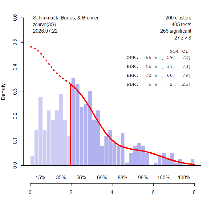
The plot confirms what the previous models suggested: there is no strong selection for statistical significance among the positive results. The observed discovery rate (ODR) is 66%, whereas zcurve3 estimates an expected discovery rate (EDR) of 46%. Thus, the point estimate suggests some selection for significance, but the confidence interval around the EDR is wide, ranging from 17% to 73%, and includes the observed rate of 66%. Consequently, the data do not provide clear evidence that non-significant results are missing. At the same time, the wide confidence interval means that substantial selection cannot be ruled out.

Zcurve3 also estimates a false discovery rate of only 6%, although the confidence interval is again wide, ranging from 2% to 25%. Thus, the results are inconsistent with an interpretation in which the large number of significant positive findings consists mostly of false positives. This is important because a grand mean close to zero can easily be misinterpreted as evidence that the significant nudging results have disappeared after correction for publication bias. That is not what these results show. They suggest that most significant results were obtained with a true effect.

Finally, zcurve3 estimates an expected replication rate (ERR) of 72%, 95% CI [60%, 79%]. This means that, under exact replication conditions, approximately seven out of ten significant positive results are expected to produce another significant result. Actual replication rates may be lower because replication studies are rarely exact and because effect sizes can vary across populations and contexts.

Replicability also increases sharply with the strength of the original evidence. The local-power estimates shown below the x-axis illustrate that studies with large z-values have a high probability of producing another significant result. Thus, even if the grand mean across all nudging interventions is close to zero, the literature clearly contains individual findings with substantial statistical evidence and high predicted replicability.

Zcurve3 also provides selection-adjusted effect-size estimates. For all positive results, the estimated mean effect is d = .37, 95% CI [.14, .60]. The confidence interval is wide because there is considerable uncertainty about how many nonsignificant positive results are missing and how small their effects are likely to be. Nevertheless, even the lower bound of the confidence interval is clearly above zero.

A statistically more precise estimate can be obtained for the significant positive results that are actually used to fit the z-curve model. Their estimated mean effect is $d=.60$, 95% CI [.47, .72]. This estimate answers a narrower question: what is the average effect size of the positive significant findings on which most published claims about successful nudges are based? For evaluating the credibility and magnitude of these claims, this conditional estimate is more informative than a grand mean that averages significant, nonsignificant, positive, and negative effects from fundamentally different interventions.

However, $d=.60$ is still only an average. Considerable heterogeneity remains among these effects, $SD=.25$, 95% CI [.13, .39]. Thus, I am not claiming that “the effect of nudging is .60.” There is no single effect of nudging. Zcurve3 provides a more meaningful average for a more narrowly defined question, but the remaining heterogeneity still needs to be examined. The next step is therefore not to replace 43 or 0 with 60 as the new answer to everything, but to identify which specific nudges produce credible effects and how large those effects are.

Zcurve3 provides a forest plot that makes it easy to identify particularly promising findings. The plot shows selection-adjusted effect-size estimates in blue, together with confidence intervals that incorporate both sampling error and uncertainty introduced by selection bias. Studies are ranked by the lower bound of their confidence interval rather than simply by their z-value or point estimate. Thus, studies rise to the top only when the data support an effect that is both reasonably large and estimated with sufficient precision. This avoids giving priority merely to very large studies that can produce impressive z-values for substantively trivial effects.

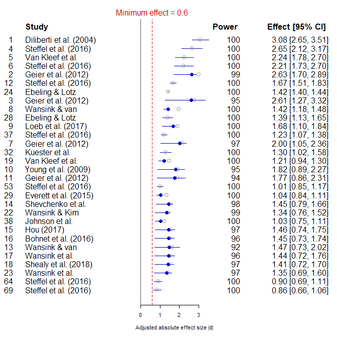
At the top of the forest plot is a study by Diliberti et al. (2004). Its z-value is outside the range used by Zcurve3 for effect-size adjustment, so the plot shows the reported effect size without correction. The estimate is $d=3.08$, an enormous standardized effect. Even the lower bound of the confidence interval is $d=2.65$. A result of this magnitude stands on its own and does not require a meta-analytic estimate. It deserves careful examination. However, an extreme meta-analytic effect-size estimate should never be trusted at face value. It could reflect a computational error in the original study, a coding error in the meta-analysis, or an unusual feature of the outcome measure. Closer inspection of the original article reveals why this estimate is so large.

Diliberti et al. manipulated portion size on different days in a cafeteria. On days when larger portions were served, customers ate more. The extraordinarily large standardized effect arose from the measure of entrée consumption. Customers who finished their entire entrée all received the same maximum value—the amount of food that had been served. This pile-up at the upper limit compressed the variance in consumption. Because a standardized effect size divides the mean difference by the standard deviation, an unusually small standard deviation can produce an extraordinarily large value of $d$.

The article also reported total caloric intake for the entire meal, an outcome with substantially more variability. The absolute difference between conditions remained large, but the standardized effect was a much more plausible $d\approx .80$. Thus, the substantive finding is robust: larger portions increased food consumption. However, the $d=3.08$ estimate exaggerates the practical magnitude of the effect because of the unusually small variance in the outcome measure. It therefore contributes artificial heterogeneity to the meta-analysis—heterogeneity caused by the construction of the effect-size measure rather than by a substantively stronger effect of the intervention. No continuous theoretical moderator of nudging should be expected to explain such an extreme value.

Once the source of an extreme effect size has been identified, it is reasonable either to replace it with a more appropriate effect-size estimate or to exclude it in a sensitivity analysis when estimating the remaining unexplained heterogeneity. This is different from deleting an outlier simply because it is extreme. The reason for treating this value differently is known: $d=3.08$ is inflated by restricted variance in the particular outcome that was selected to represent the study.

Another question is whether a portion-size manipulation should be included in a meta-analysis of nudging in the first place. Maier et al. (2022) tried to address heterogeneity by conducting separate analyses for six broad domains. For the food domain, the Bayes factor favored a nonzero average effect, although the evidence was weak. In the other five domains, the Bayes factors pointed toward a mean of zero to varying degrees ($BF_{01}>1$), although only three reached the conventional 3:1 threshold for moderate evidence. Nevertheless, these results have been summarized as showing that “using more precise estimates, the results revealed evidence against the efficacy of nudges in most domains” (PsyPost). This statement illustrates how easily results from RoBMA can be misinterpreted. A Bayes factor concerns the average effect within a domain. Even a Bayes factor of 1000:1 in favor of a mean of zero would not show that nudges have no effects when the same model estimates substantial heterogeneity. Thus, all reported means should be reported with the estimate of heterogeneity to avoid this misinterpretation.

Maybe the old criticism that heterogeneous meta-analyses compare apples and oranges was right after all (Sharpe, 1997). If apple studies and orange studies have systematically different effect sizes, their average is informative about neither apples nor oranges. Combining them merely creates heterogeneity. When a moderator analysis eventually discovers the apple-orange distinction, researchers report separate estimates for apples and oranges. But they could have done that from the beginning, without first mixing them together and reporting an average effect of “fruit.”

Another question is whether a portion-size manipulation should be included in a meta-analysis of nudging in the first place. Maier et al. (2022) also examined six different domains and found support for an average effect in the food domain. However, their Bayesian statistic pointed towards evidence for the null hypothesis to various degrees (BF01 > 1) in five other domains. This finding has been reported as “using more precise estimates, the results revealed evidence against the efficacy of nudges in most domains” (psypost.org). This claims illustrates how confusing RoBMA results can be and how they are easily misunderstood. Most importantly, even a Bayes-Factor of 1000:1 in favor of a mean of zero in these analysis does not justify the claim that there is no effect when studies also show heterogeneity.

Maybe the old criticism that heterogeneous meta-analyses are like comparisons of apples and oranges was right after all (Sharpe, 1997). If apple studies and orange studies have systematically different effect sizes, their average is informative about neither apples nor oranges. Combining them merely creates heterogeneity. When a moderator analysis eventually discovers the apple-orange distinction, researchers report separate estimates for apples and oranges. But they could have done that from the beginning, without first mixing them together and reporting an average effect of “fruit.”Maybe the old criticism that heterogeneous meta-analyses are like comparisons of apples and oranges was right after all (Sharpe, 1997). If apple studies and orange studies have systematically different effect sizes, their average is informative about neither apples nor oranges. Combining them merely creates heterogeneity. When a moderator analysis eventually discovers the apple-orange distinction, researchers report separate estimates for apples and oranges. But they could have done that from the beginning, without first mixing them together and reporting an average effect of “fruit.”

This points to an even more fundamental problem with averaging positive and negative population effects. Suppose eating an apple a day keeps the doctor away, whereas eating an orange a day makes people sick. Both are real effects. They receive positive or negative signs only because of a convention about which direction is desirable or consistent with a theoretical prediction. If the two effects are equal in magnitude but opposite in sign, their average is zero. But this does not imply that there is no effect. It implies that two real effects cancel mathematically when they are averaged. The scientifically useful conclusion would be to eat apples and avoid oranges—not that “fruit has no effect.”

Meta-analyses in medicine often take a much narrower approach. Rather than combining fundamentally different treatments and outcomes under a broad label, they typically focus on closely related interventions, comparable control conditions, similar populations, and clearly defined outcomes. As a result, many clinically informative meta-analyses contain fewer than 20 studies. That may sound less impressive than a meta-analysis based on more than 200 publications, but in meta-analysis, more is not necessarily better. Often, less is more—except when it comes to the sample sizes of the original studies. A meta-analysis gains credibility from the comparability of the studies, not from the sheer number of papers thrown into it.

The broader lesson is that methods designed to evaluate the credibility of published research must themselves be evaluated critically. Meta-scientists are subject to the same incentives as other scientists, and sophisticated statistical methods do not eliminate the need to examine assumptions, alternative explanations, and the full implications of a fitted model. In this case, focusing on a grand mean close to zero obscured substantial heterogeneity, little evidence of selection for statistical significance, and considerable evidence for positive and potentially replicable effects. A credibility revolution should make scientific claims more carefully calibrated, not merely replace one headline number with another.

Selected References

Bartoš, F., & Schimmack, U. (2022). Z-curve 2.0: Estimating replication rates and discovery rates. Meta-Psychology, 6, Article e0000130. https://doi.org/10.15626/MP.2022.2981

Maier, M., Bartoš, F., Stanley, T. D., Shanks, D. R., Harris, A. J. L., & Wagenmakers, E.-J. (2022). No evidence for nudging after adjusting for publication bias. Proceedings of the National Academy of Sciences, 119(31), e2200300119. https://doi.org/10.1073/pnas.2200300119

Sharpe D. (1997). Of apples and oranges, file drawers and garbage: why validity issues in meta-analysis will not go away. Clinical psychology review, 17(8), 881–901. https://doi.org/10.1016/s0272-7358(97)00056-1

Szászi, B., Higney, A., Charlton, A., Gelman, A., Ziano, I., Aczel, B., Goldstein, D. G., Yeager, D. S., & Tipton, E. (2022). No reason to expect large and consistent effects of nudge interventions. Proceedings of the National Academy of Sciences, 119(31), e2200732119. https://doi.org/10.1073/pnas.2200732119