I was fortunate enough to read Jacob Cohen’s articles early on in my career to avoid many of the issues that plague psychological science. One of his important lessons was that it is better to test a few (or better one) hypothesis in one large sample (Cohen, 1990) than to conduct many tests in small samples.

The reason is simple. Even if a theory makes a correct prediction, sampling error may produce a non-significant result, especially in small samples where sampling error is large. This type of error is known as type-II error, beta, or a false negative. The probability of obtaining the desired and correct outcome of a significant result, when a hypothesis is true is called power. The problem of testing multiple hypotheses is that the cumulative or total power of finding evidence for all correct hypotheses decreases with the number of tests. Even if a single test has 80% power (i.e., the probability of a significant result for a correct hypothesis is 80 percent), the probability of providing evidence for 10 correct hypotheses is only .8^10 = .11%. The expected value is that 2 of the 10 tests produce a type-II error (Schimmack, 2012).

Cohen (1961) also noted that the average power of statistical tests is well below 80%. For a medium/average effect size, power was around 50%. Now imagine that a researcher tests 10 true hypotheses with 50% power. The expected value is that 5 tests produce a significant result (p < .05) and 5 studies produce a type-II error (p > .05). The interpretation of the article will focus on the significant results, but they were selected basically by a coin flip. The next study will produce a different set of 5 significant studies.

To avoid type-II errors researchers could conduct a priori power analysis to ensure that they have enough power. However, this is rarely done with the explanation that a priori power analysis requires knowledge about the population effect size, which is unknown. However, it is possible to estimate the typical power of studies by keeping track of the percentage of significant results. Because power determines the rate of significant results, the rate of significant results is an estimate of average power. The main problem with this simple method of estimating power is that researchers often do not report all of their results. Especially before the replication crisis became apparent, psychologists tended to publish only significant results. As a result, it is largely unknown how much power actual studies in psychology have and whether power increased since Cohen (1961) estimated power to be around 50%.

Here I illustrate a simple way to estimate actual power of studies with a recent multi-study article that reported a total of 184 significance tests (more were reported in a supplement, but were not coded)! Evidently, Cohen’s important insights remain neglected, especially in journals that pride themselves on rigorous examination of hypotheses (Kardas, Kumar, & Epley, 2021).

Figure 2 shows the first rows of the coding spreadsheet (Spreadsheet).

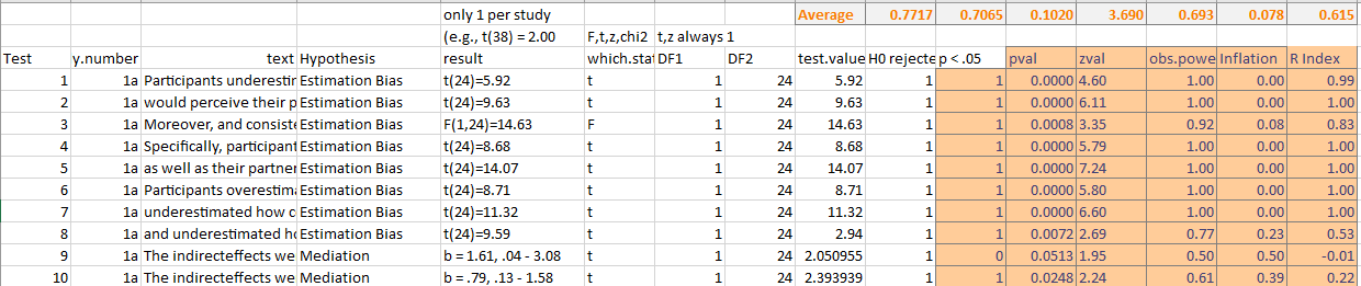
Each row shows one specific statistical test. The column “HO rejected” reflects how authors interpreted a result. Broadly this decision is based on the p < .05 rule, but sometimes authors are willing to treat values just above .05 as sufficient evidence which is often called marginal significance. The column p < .05 strictly follows the p < .05 rule. The averages in the top row show that there are 77% significant results using authors’ rules and 71% using the p < .05 rule. This shows that 6% of the p-values were interpreted as marginally significant.

All test-values or point estimates with confidence intervals are converted into exact two-sided p-values. The two-sided p-values are then converted into z-scores using the inverse normal formula; z = -qnorm(2). Observed power is then estimated for the standard criterion of significance; alpha = .05, which corresponds to a z-score of 1.96. The formula for observed power is pnorm(z, 1.96). The top row shows that mean observed power is 69%. This is close to the 71% percentage with the strict p < .05 rule, but a bit lower than the 77% when marginally significant results are included. This simple comparison shows that marginally significant results inflate the percentage of significant results.

The inflation column keeps track of the consistency between the outcome of a significance test and the power estimate. When power is practically 1, a significant result is expected and inflation is zero. However, when power is only 60%, there is a 40% chance of a type-II error and authors were lucky if they got a significant result. This can happen in a single test, but not in the long run. Average inflation is a measure of how lucky authors were if they got more significant results than the power of their studies allows. Using the authors 77% success rate and estimated power of 69%, we have an inflation of 8%. This is a small bias, and we already saw that interpretation of marginal results accounts for most of it.

The last column is called the Replication Index (R-Index). It simply subtracts the inflation from the observed power estimate. The reason is that observed power is an inflated estimate of power when there are too many significant results. The R-Index is called an index because the formula is just an approximate correction for selection for significance. Later I show the results with a better method. However, the Index can clearly distinguish between junk science (R-Index below 50) and credible evidence. Based on the present results, the R-Index of 62 shows that the article reported some credible findings. Moreover, the R-Index now underestimates power because the rate of p-values below .05 is consistent with observed power. The inflation is just due to the interpretation of marginal results as significant. In short, the main conclusion from this simple analysis of test statistics in a single article is that the authors conducted studies with an average power of about 70%. This is expected to produce type-II errors, sometimes with p-values close to .05 and sometimes with p-values well above .1. This could mean that nearly a quarter of the published results are type-II errors.

but what about type-I errors?

Cohen was concerned about the problem that many underpowered studies fail to reject true hypotheses. However, the replication crisis shifted the focus from false negative results to false-positive results. An influential article by Simmons et al. (2011) suggested that many if not most published results might be false positive results. The authors also developed a statistical tool that examines whether a set of significant results is entirely based on false positive results called p-curve. The next figure shows the output of the p-curve app for the 130 significant results (only significant results are considered because p-values greater than .05 cannot be false positives).

The graph shows that there a lot more p-values below .01 (78%) than p-values between .04 and .05 (2%). This distribution of p-values is inconsistent with the hypothesis that all significant results are false positives. In addition, the program estimates that the average power of the 130 studies with significant results is 99%! As a result, there can be no false positives that would produce an estimate of 5% power. It is noteworthy that the p-curve analysis did not spot the inflation of significant results by interpreting marginally significant results because these results are omitted from the p-curve analysis. It is rather unlikely that the average power of studies is 99%. In fact, simulation studies have shown that the power estimates of p-curve are often inflated when studies are heterogeneous (Brunner, 2018; Brunner & Schimmack, 2020). The p-curve authors are aware of this bug, but have done nothing to fix it (Datacolada, 2018).

A better statistical method to analyze p-values is z-curve, which relies on the z-scores that were obtained from the p-values in the spreadsheet. However, the z-curve package for R can also read p-values. The next Figure shows a histogram of all 184 (significant and non-significant) values up to a value of 6. Values over 6 are not shown and are all treated as studies with perfect power.

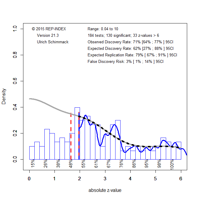
The expected discovery rate corresponds to the power estimate in p-curve. It is notably lower than 99% and the 95%CI excludes a value of 99%. This finding simply shows once again that p-curve estimates are inflated.

The observed discovery rate is simply the same percentage that was computed on the spreadsheet using a strict p < .05 rule. The expected discovery rate is an estimate of the average power for all studies, including non-significant results that is corrected for any potential inflation. It is 62%, which matches the R-Index in the spreadsheet.

The comparison of the observed discovery rate of 71% and the expected discovery rate of 62% suggests that there is some overreporting of significant results. However, the 95%CI around the EDR estimate ranges from 27% to 88%. Thus, sampling error alone may explain this discrepancy.

An EDR of 62% implies that only a small number of significant results can be false positives. The point estimate is just 2%, but the 95%CI allows for up to 14% false positives. Thus, the reported results are unlikely to be false positives, but effect sizes could be inflated because selection for significance with modest power inflates effect size estimates.

There is also notable evidence of heterogeneity. The distribution of z-scores is much flatter than a standard normal distribution that is expected if all studies had the same power. This means that some results might be more credible than others. Therefore I conducted some moderator analyses.

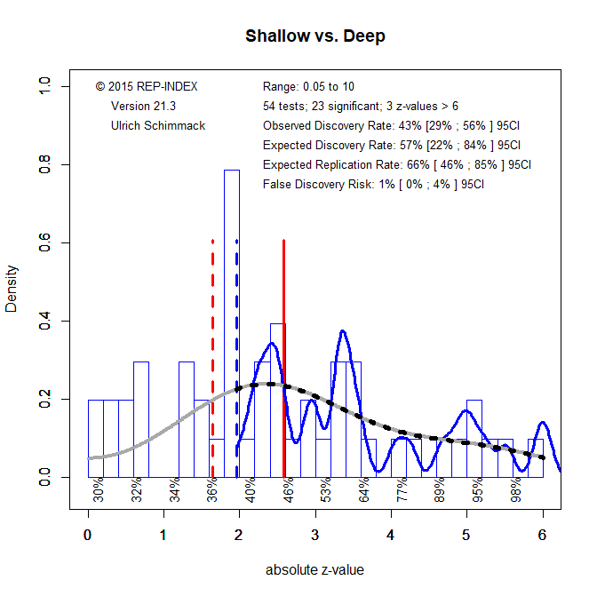
One key hypothesis in the article was that shallow and deep conversations differ in important ways. Several studies tested this by comparing shallow and deep conversations. Fifty-four analyses included a contrast between shallow and deep conversations as a main effect or in an interaction. The expected replication rate is unchanged. The expected discovery rate is a bit higher, but surprisingly, the observed discovery rate is lower. Visual inspection of the z-curve plot shows an unusually high number of marginally significant results. This is further evidence to distrust marginally significant results. However, overall these results suggest that shallow and deep conversations differ.

Several analyses tested mediation, which can require large samples to have adequate power. Not surprisingly, the 39 mediation tests have only a replication rate of 53%. There is also some suggestion of bias, with an observed discovery rate of 51% and an expected discovery rate of only 25%, but the 95%CI around the point estimate is wide and includes 51%. The low expected discovery rate implies that the false discovery risk is 16%, which is unacceptably high.

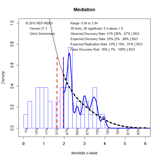
One solution to the high false discovery risk is to lower the criterion for significance. The next conventional level is alpha = .01. The next figure shows the results for this criterion value (the red solid line has moved to z = 2.58.

Now the observed discovery rate is in line with the expected discovery rate (28% vs. 27%) and the false discovery risk has been lowered to 3%. However, the expected replication rate (for alpha = .01) is only 36%. Thus, follow-up studies need to increase sample sizes to replicate these mediation effects.

Conclusion

A post-hoc power-analysis of this recent article shows that psychologists still have not learned Cohen’s lesson that he shared in 1990 (more than 30 years ago). Conducting many significance tests with modest statistical power produces a confusing pattern of significant and non-significant results that is strongly influenced by sampling error. Rather than reporting results of individual studies, the authors should have reported meta-analytic results for tests of the same hypothesis. However, to end on a positive note, the studies are not p-hacked and the risk of false positives is low. Thus, the results provide some credible findings that can be used to conduct confirmatory tests of the hypothesis that deeper conversations are more awkward, but also more rewarding. I hope these analyses show that a deep dive into the statistical results reported in an article can also be rewarding.