In this mini-tutorial, I discuss the relationship between p-values and z-scores. Although the standard normal distribution is a staple for intro stats, it plays a minor role when researchers conduct actual research with t-tests, F-tests and often only look up test statistics and p-values without thinking about the underlying sampling distributions of their test statistics. A better understanding of p-values and z-scores is needed because new statistical methods rely on meta-analyses of p-values or z-scores to make claims about the quality of psychological research.

Basic Introduction

Let’s assume that researchers would use z-tests to analyze their data and convert z-tests into p-values to determine whether a result is statistically significant, p < .05. In the statistics program R, the conversion of a z-score into a p-value uses the command pnorm(z, mean, sd). For significance testing we want to know how extreme the observed z-score is relative to the null-hypothesis, which is defined by a standard normal distribution with mean = 0, and sd = 1). So, we would use the command pnorm(z, mean=0, sd=1). Because the standard normal is the default assumption, we can also simply request the p-value with pnorm(z).

However, using this command will produce some strange results. For example, if we observed a z-score of 2.5, we obtain a p-value of .99, which would suggest that our result is not significant p > .05. The problem is that the default option in R is to provide the area under the standard normal distribution on the left side of the z-score. So, we see that 99% of the distribution is on the left side, the lower tail, and only 1% is on the right side, the upper tail. With only 1% in the upper tail, we can claim a significant result, p < .05.

pnorm(2.5)
[1] 0.9937903

There are various options to obtain the p-value we really want. One option is to write pnorm(2.5, lower.tail-FALSE), which gives use p = .01.

pnorm(2.5, lower.tail=FALSE)
[1] 0.006209665

A simpler option is to make use of the symmetry of the standard normal distribution and simply turn the positive z-score into a negative z-score.

pnorm(-2.5)
[1] 0.006209665

Yet another option is to subtract the lower tail from 1.

1-pnorm(2.5)
[1] 0.006209665

So, we see that a z-score of 2.5 is statistically significant with p < .05. However, z-scores are two-sided. That is they have positive and negative values. What if we had observed a z-score of -2.5. Would that also be significant? As we can see, the answer is no. The reason is that we are conducting one-tailed tests, where only positive deviations from H0 can be used to reject the null-hypothesis.

1-pnorm(-2.5)
[1] 0.9937903

Typically, psychologists prefer two-tailed tests, which is the default for F-tests that ignore the sign of an effect. To make the sign irrelevant, we can simply use the absolute z-score to obtain our upper tail p-value.

1-pnorm(abs(-2.5))
[1] 0.006209665

Now we get the same p-value that we obtained for z = 2.5. However, checking both tails doubles the risk of a type-I error. Therefore, we have to double the p-value, if we want to conduct a two-tailed test.

(1-pnorm(abs(-2.5)))*2
[1] 0.01241933

Multiple p-values

Psychologists are familiar with effect size meta-analysis. However, before effect size meta-analysis became common, meta-analyses were carried out with p-values or z-scores. Fisher not only invented p-values, he also introduced a method to combine p-values from multiple studies. Meta-analysis of p-values have encountered a renaissance in psychology with the introduction of p-curve, which is essentially a histogram of statistically significant p-values. Importantly, p-curve is based on two-tailed p-values, as I will demonstrate below.

Assume that we have a large set of z-tests from 1000 studies, but all 1000 studies tested a true null-hypothesis. As a result, we would expect that the 1000 z-scores follow the sampling distribution of a standard normal distribution.

z = rnorm(1000)
hist(z,freq=FALSE,xlim=c(-3,3),ylim=c(0,.5),ylab=”Density”)
par(new=TRUE)
curve(dnorm(x),-3,3,ylim=c(0,.5),ylab=””)

After we convert the z-scores into ONE-TAILED p-values, we see that they follow a uniform distribution.

p = pnorm(-z)

The same is true for TWO-TAILED p-values

p = (1-pnorm(abs(z)))*2
hist(p)p = pnorm(abs(z))*2
hist(p)

However, this is only true for the special case, when the null-hypothesis is true. When the null-hypothesis is false, the histograms of p-values (p-curves) differ dramatically.

z = rnorm(1000,1,3)
hist(z,freq=FALSE,xlim=c(-9,9),ylim=c(0,.5),ylab=”Density”)
par(new=TRUE)
curve(dnorm(x,1,3),-9,9,ylim=c(0,.5),ylab=””)

For the one-tailed p-values the distribution is bimodal. The reason is that null-effects are represented by p-values of .5. As we simulated many extreme positive and extreme negative deviations from 0, we have more p-values in the tails, close to 0 and close to 1, than p-values in the middle. Evidently, p-values are not just decreasing from 0 to 1.

However, if we compute two-tailed p-values, the distribution of p-values shows decreasing frequencies from 0 to 1.

In sum, it is important to think about the tails of a p-value. One-tailed p-values should be used when the sign of a test is meaningful. For example, in a meta-analysis of studies that tested the same hypothesis. In this case, we need to obtain p-values from test statistics that have a direction (z-scores, t-value) and we cannot use test statistics that remove information about the direction of a test (F-values, chi-square values). However, if we do not care about the sign of an effect, we should use two-tailed p-values because we only care about the strength of evidence against the null-hypothesis.

Going from p-values to z-scores

Meta-analyses of p-values can use p-values that are based on different test statistics (t-tests, F-tests, etc.). The reason is that all p-values have the same meaning. A p-value of .02 from a z-test provides the same information as a p-value of .02 from a t-test. However, p-values have an undesirable distribution. A solution to this problem is to convert p-values into values that follow a distribution with more desirable characteristics. The most desirable distribution is the standard normal distribution. Thus, we can use z-scores as a common metric to compare results of different studies (Stauffer et al., 1938).

However, we have to think again about the tails of p-values when we convert p-values into z-scores. If all p-values are one-tailed p-values, we can simply convert our upper-tail p-values into z-scores using the qnorm command. Simulating a uniform distribution of p-values and converting the p-values into z-scores gives us the standard normal distribution centered over 0.

p = runif(1000,0,1)
z = qnorm(p,lower.tail=FALSE)

However, things are more complicated with TWO-TAILED p-values as shown in the diagram below. First, we simulated a set of z-tests as before. We then convert the results into two-tailed p-values and convert them back. The conversion has to take into account that we doubled p-values to take into account two-tailed testing. So, now we need to half the p-values before we convert from p to z.

z = rnorm(1000,1,3)
p = (1-pnorm(abs(z)))*2
qz = -qnorm(p/2)
hist(z,freq=FALSE,xlim=c(-9,9),ylim=c(0,.5),ylab=”Density”,main=”Z-curve”,xlab=”z-value”)
par(new=TRUE)
hist(qz,freq=FALSE,xlim=c(-9,9),ylim=c(0,.5),ylab=”Density”,col=”red”,density=10,main=””,xlab=””)

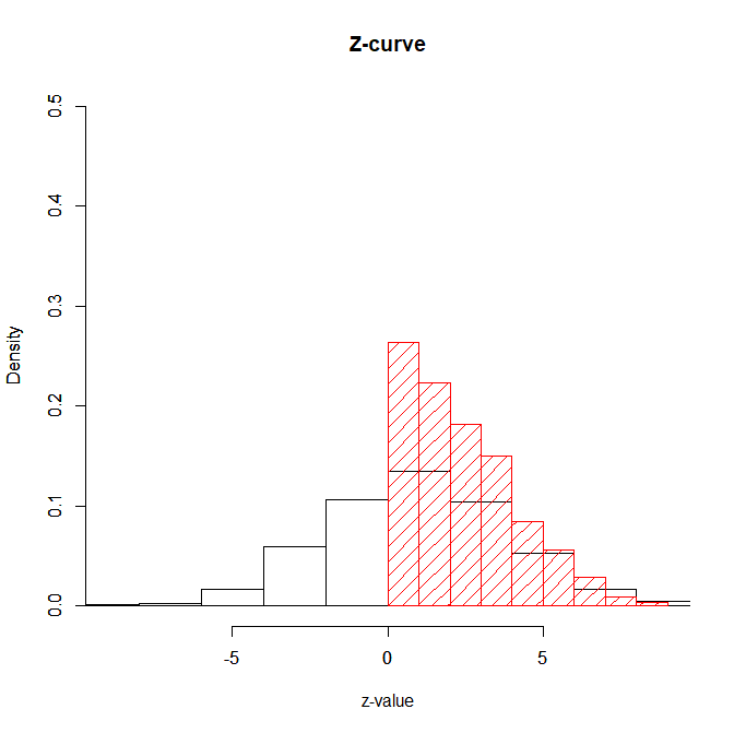
However, we see that the distribution of the original z-scores (black) differs form the distribution of the z-scores obtained from two-tailed p-values. The difference is that the converted z-scores do not have negative values. They are ABSOLUTE z-scores because the computation of two-tailed p-values erased information about the sign of a test. A low p-value could have been obtained from a high positive or a high negative z-score. To see this we can compare the converted z-scores to the absolute values of the original z-scores.

hist(abs(z),freq=FALSE,xlim=c(0,9),ylim=c(0,.5),ylab=”Density”,main=”Z-curve”,xlab=”z-value”,density=20)
par(new=TRUE)
hist(qz,freq=FALSE,xlim=c(0,9),ylim=c(0,.5),ylab=”Density”,col=”red”,density=10,main=””,xlab=””)

In sum, if we convert one-tailed p-values into z-scores, we retain information about the sign of an effect and the sampling error follows a standard normal distribution. However, if we use two-tailed p-values and convert them into z-scores, the distribution of z-scores is truncated at zero and only positive z-scores can be observed. Sampling error no longer follows a standard normal distribution.

A Minor Technical Problem

As noted before, p-values have an undesirable distribution. A z-score of 1 corresponds to a two-tailed p-value of p = .32. A z-score of 2 corresponds to a p-value of .05. A z-score of 3 corresponds to a p-value of p = .003. A z-score of 4 corresponds to a p-value of .0001. A z-score of 5 corresponds to a p-value of .000001. The number of zeros behind the decimal point increases quickly and at some point, rounding errors make it impossible to convert p-values into z-scores.

p = (1-pnorm(8.3))*2
-qnorm(p/2)
[1] Inf

All p-values for z-scores greater than 8.2 are treated as 0 and are converted into a z-score of infinity. To avoid this problem, R provides the option to use log p-values. Using the log.p option makes it possible to convert a z-score of 10 into p-value and to retrieve the value of 10 after converting the p-value into a log and to obtain the correct z-score.

p = pnorm(10,lower.tail=FALSE)*2
p
[1] 0.00000000000000000000001523971
-qnorm(log(p) – log(2),log.p=TRUE)
[1] 10

Does and Don’ts

Just like meta-analysis of p-values has seen a renaissance, meta-analysis of z-scores has also seen renewed attention. Jerry Brunner and I developed z-curve to estimate mean power of a set of studies that were selected for significance and have heterogeneity in power as a result of heterogeneity in sample sizes and effect sizes (Brunner & Schimmack, 2018). Z-curve first converts all observed test-statistics into TWO-TAILED p-values and then converts two-tailed p-values into ABSOLUTE Z-SCORES. The method then fits several TRUNCATED standard normal distributions to the data to obtain estimates of statistical power.

Another method is the Bayesian Mixture Model (BMM) that aims to estimate the percentage of false positives in a set of studies. However, the BMM model has several deficiencies in the conversion process from p-values to z-scores.

First, it uses the formula for ONE-TAILED p-values when the input are TWO-TAILED p-values.

Second, it converts upper-tail p-values into z-scores using the formula for lower-tail p-values.

z = qnorm(p).

As a result, the distribution of z-scores obtained from p-values that were produced by z-tests differs from the distribution of the actual z-tests.

z = rnorm(10000,1)
p = (1-pnorm(abs(z)))*2

qz = qnorm(p) #BMM transformation
hist(z,freq=FALSE,xlim=c(-5,5),ylim=c(0,.5),ylab=”Density”,main=”Z-curve”,xlab=”z-value”)
par(new=TRUE)
hist(qz,freq=FALSE,xlim=c(-5,5),ylim=c(0,.5),ylab=”Density”,col=”red”,density=10,main=””,xlab=””)
par(new=TRUE)
curve(dnorm(x,1),-5,5,ylim=c(0,.5),ylab=””)

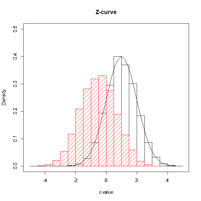
qz = -qnorm(p) #FLIPPED BMM transformation

Even if we correct for the sign error and flip the distribution, the reproduced distribution differs from the original distribution because TWO-TAILED p-values are converted into z-scores using the formula for ONE-TAILED p-values.

In conclusion, it is important to think about the tails of p-values. One-tailed p-values are not identical to two-tailed p-values. Using the formula for one-tailed p-values with two-tailed p-values distorts the information that is provided by the actual data. Two-tailed p-values do not contain information about the sign of an effect. Converting them into z-scores produces absolute z-scores that reflect the strength of evidence against the null-hypothesis without information about the direction of an effect.

Conclusion

P-values and z-scores contain valuable information about the results of studies. Both p-values and z-scores provide a common metric to compare results of studies that used different test statistics or differed in sample sizes (and degrees of freedom). Meta-analysts can use standardized effect sizes, p-values, or z-scores. P-values and z-scores can be transformed into each other without further information about sample sizes. However, to convert them properly, we have to take into account whether p-values tested a one-tailed or a two-tailed hypothesis. For one-tailed tests, the null-hypothesis corresponds to a p-value of .5 with values of 0 and 1 corresponding to very strong (infinite) evidence against the null-hypothesis. For two-tailed tests, p-values of 1 correspond to the null-hypothesis and a value of 0 corresponds to infinite evidence against the null-hypothesis. For z-scores a value of 0 corresponds to the null-hypothesis and increasing values in either direction provide evidence against it. Thus, one-tailed p-values correspond to z-scores with p = 0 corresponding to z = inf, p = .5 corresponding to z = 0, and p = 1 corresponding to z = -inf. In contrast, two-tailed p-values only provide information about strength of evidence and a p-value of 1 corresponds to z = 0, while a p-value of 0 corresponds to z = inf. Any meta-analysis with z-scores requires a transformation into p-values to create a common metric. The conversion of p-values into z-scores for this purpose should take into account whether p-values are one-tailed or two-tailed. Converting two-tailed p-values into z-scores using the formula for one-tailed p-values may lead to false conclusions in a meta-analysis of z-scores.