The logic of null-hypothesis significance testing is straightforward (Schimmack, 2017). The observed signal in a study is compared against the noise in the data due to sampling variation. This signal to noise ratio is used to compute a probability; p-value. If this p-value is below a threshold, typically p < .05, it is assumed that the observed signal is not just noise and the null-hypothesis is rejected in favor of the hypothesis that the observed signal reflects a true effect.
NHST aims to keep the probability of a false positive discovery at a desirable rate. With p < .05, no more than 5% of ALL statistical tests can be false positives. In other words, the long-run rate of false positive discoveries cannot exceed 5%.
The problem with the application of NHST in practice is that not all statistical results are reported. As a result, the rate of false positive discoveries can be much higher than 5% (Sterling, 1959; Sterling et al., 1995) and statistical significance no longer provides meaningful information about the probability of false positive results.
In order to produce meaningful statistical results it would be necessary to know how many statistical tests were actually performed to produce published significant results. This set of studies includes studies with non-significant results that remained unpublished. This set of studies is often called researchers’ file-drawer (Rosenthal, 1979). Schimmack and Brunner (2016) developed a statistical method that estimates the size of researchers’ file drawer. This makes it possible to correct reported p-values for publication bias so that p-values resume their proper function of providing statistical evidence about the probability of observing a false-positive result.
The correction process is first illustrated with a powergraph for statistical results reported in 103 journals in the year 2016 (see 2016 Replicability Rankings for more details). Each test statistic is converted into an absolute z-score. Absolute z-scores quantify the signal to noise ratio in a study. Z-scores can be compared against the standard normal distribution that is expected from studies without an effect (the null-hypothesis). A z-score of 1.96 (see red dashed vertical line in the graph) corresponds to the typical p < .05 (two-tailed) criterion. The graph below shows that 63% of reported test statistics were statistically significant using this criterion.
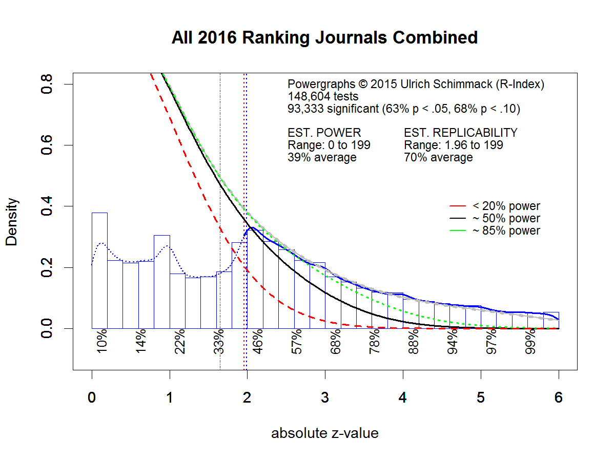
Powergraphs use a statistical method, z-curve (Schimmack & Brunner, 2016) to model the distribution of statistically significant z-scores (z-scores > 1.96). Based on the model results, it estimates how many non-significant results one would expect. This expected distribution is shown with the grey curve in the figure. The grey curve overlaps with the green and black curve. It is clearly visible that the estimated number of non-significant results is much larger than the actually reported number of non-significant results (the blue bars of z-scores between 0 and 1.96). This shows the size of the file-drawer.
Powergraphs provide important information about the average power of studies in psychology. Power is the average probability of obtaining a statistically significant result in the set of all statistical tests that were conducted, including the file drawer. The estimated power is 39%. This estimate is consistent with other estimates of power (Cohen, 1962; Sedlmeier & Gigerenzer, 1989), and below the acceptable minimum of 50% (Tversky and Kahneman, 1971).
Powergraphs also provide important information about the replicability of significant results. A published significant result is used to support the claim of a discovery. However, even a true discovery may not be replicable if the original study had low statistical power. In this case, it is likely that a replication study produces a false negative result; it fails to affirm the presence of an effect with p < .05, even though an effect actually exists. The powergraph estimate of replicability is 70%. That is, any randomly drawn significant effect published in 2016 has only a 70% chance of reproducing a significant result again in an exact replication study.
Importantly, replicability is not uniform across all significant results. Replicabilty increases with the signal to noise ratio (Open Science Collective, 2015). In 2017 powergraphs were enhanced by providing information about the replicability for different levels of strength of evidence. In the graph below, z-scores between 0 and 6 are divided into 12 categories with a width of 0.5 standard deviations (0-0.5, 0.5-1, …. 5.5-6). For significant results, these values are the average replicability for z-scores in the specified range.
The graph shows a replicability estimate of 46% for z-scores between 2 and 2.5. Thus, a z-score greater than 2.5 is needed to meet the minimum standard of 50% replicability. More important, these power values can be converted into p-values because power and p-values are monotonically related (Hoenig & Heisey, 2001). If p < .05 is the significance criterion, 50% power corresponds to a p-value of .05. This also means that all z-scores less than 2.5 correspond to p-values greater than .05 once we take the influence of publication bias into account. A z-score of 2.6 roughly corresponds to a p-value of .01. Thus, a simple heuristic for readers of psychology journals is to consider only p < .01 values as significant, if they want to maintain the nominal error rate of 5%.
One problem with a general adjustment is that file drawers can differ across journals or authors. The adjustment based on the general publication bias across journals will penalize authors who invest resources into well-designed studies with high power and it will fail to adjust fully for the effect of publication bias for authors that conduct many underpowered studies that capitalize on chance to produce significant results. It is widely recognized that scientific markets reward quantity of publications over quality. A personalized adjustment can solve this problem because authors with large file drawers will get a bigger adjustment and many of their nominally significant result will no longer be significant after an adjustment for publication bias has been made.
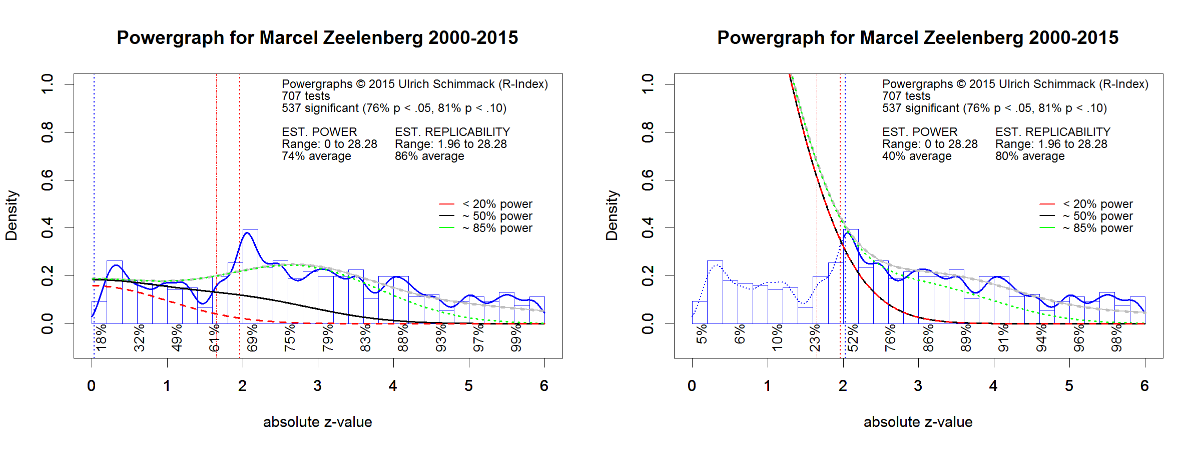
I illustrate this with two real world examples. The first example shows the powergraph of Marcel Zeelenberg. The left powergraph shows a model that assumes no file drawer. The model fits the actual distribution of z-scores rather well. However, the graph shows a small bump of just significant results (z = 2 to 2.2) that is not explained by the model. This bump could reflect the use of questionable research practices (QRPs)but it is relatively small (as we will see shortly). The graph on the right side uses only statistically significant results. This is important because only these results were published to claim a discovery. We see how the small bump leads has a strong effect on the estimate of the file drawer. It would require a large set of non-significant results to produce this bump. It is more likely that QRPs were used to produce it. However, the bump is small and overall replicability is higher than the average for all journals. We also see that z-scores between 2 and 2.5 have an average replicability estimate of 52%. This means no adjustment is needed and p-values reported by Marcel Zellenberg can be interpreted without adjustment. Over the 15 year period, Marcel Zellenberg reported 537 significant results and we can conclude from this analysis that no more than 5% (27) of these results are false positive results.
A different picture emerges for the powergraph based on Ayalet Fishbach’s statistical results. The left graph shows a big bump of just significant results that is not explained by a model without publication bias. The right graph shows that the replicabilty estimate is much lower than for Marcel Zeelenberg and for the analysis of all journals in 2016.
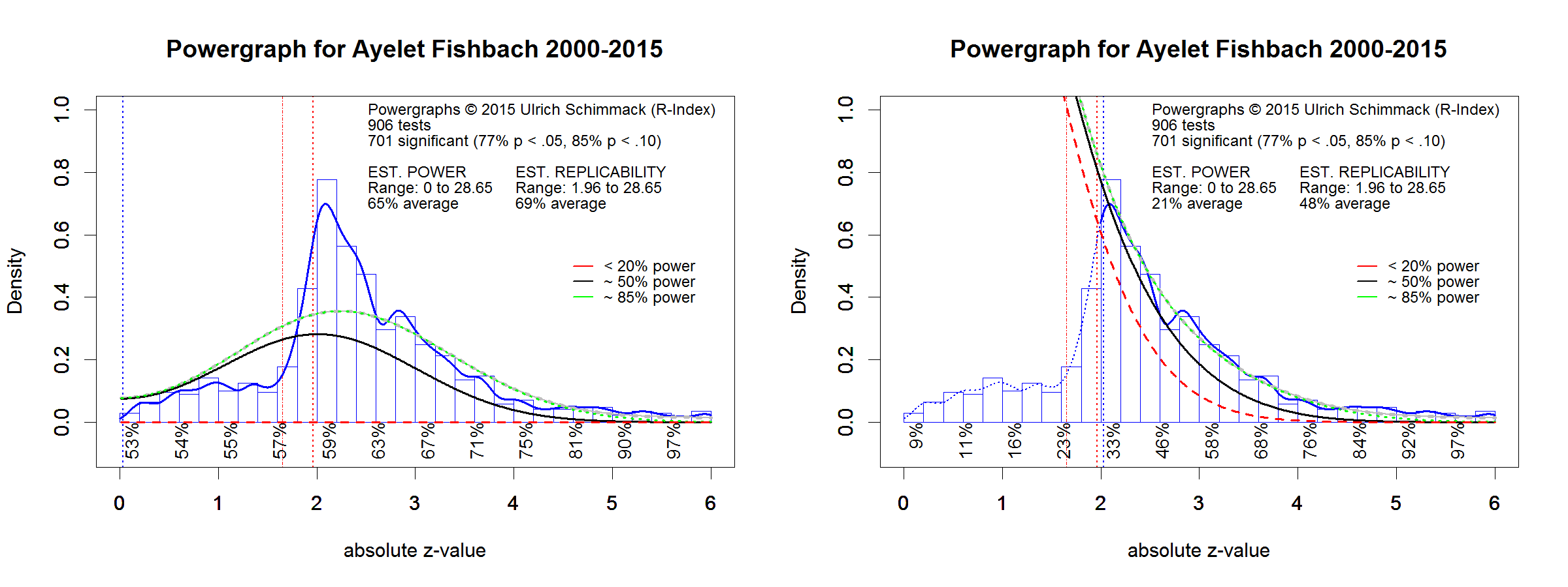
The average replicabilty estimate for z-values between 2 and 2.5 is only 33%. This means that researchers are unlikely to obtain a significant result, if they attempted an exact replication study of one of these findings. More important, it means that p-values adjusted for publication bias are well above p > .05. Even z-scores in the 2.5 to 3 band average only a replicabilty estimate of 46%. This means that only z-scores greater than 3 produce significant results after the correction for publication bias is applied.
Non-Significance Does Not Mean Null-Effect
It is important to realize that a non-significant result does not mean that there is no effect. Is simply means that the signal to noise ratio is too weak to infer that an effect was present. it is entirely possible that Ayelet Fishbach made theoretically correct predictions. However, to provide evidence for her hypotheses, she conducted studies with a high failure rate and many of these studies failed to support her hypotheses. These failures were not reported but they have to be taken into account in the assessment of the risk of a false discovery. A p-value of .05 is only meaningful in the context of the number of attempts that have been made. Nominally a p-value of .03 may appear to be the same across statistical analysis. But the real evidential value of a p-value is not equivalent. Using powergraphs to equate evidentival value, a p-value of .05 published by Marcel Zeelenberg is equivalent to a p-value of .005 (z = 2.8) published by Ayelet Fischbach.
The Influence of Questionable Research Practices
Powergraphs assume that an excessive number of significant results is caused by publication bias. However, questionable research practices also contribute to the reporting of mostly successful results. Replicability estimates and the p-value ajdustment for publication bias may itself be biased by the use of QRPs. Unfortunately, this effect is difficult to predict because different QRPs have different effects on replicability estimates. Some QRPs will lead to an overcorrection. Although this creates uncertainty about the right amount of adjustment, a stronger adjustment may have the advantage that it could deter researchers from using QRPs because it would undermine the credibility of their published results.
Conclusion
Over the past five years, psychologists have contemplated ways to improve the credibitliy and replicability of published results. So far, these ideas have yet to show a notable effect on replicability (Schimmack, 2017). One reason is that the incentive structure rewards number of publications and replicability is not considered in the review process. Reviewers and editors treat all p-values as equal, when they are not. The ability to adjust p-values based on the true evidential value that they provide may help to change this. Journals may lose their impact once readers adjust p-values and realize that many nominally significant result are actually not statistically significant after taking publication bias into account.