Social science is undermined by slippery language and sloppy measurement. The term happiness (singular) has led to a lot of confusion about the meaning of happiness or its twin wellbeing. It seems to imply that there is one happiness, one way to have high wellbeing, and one way to have a good life. Philosophers have tried to define this elusive construct without success. Not a problem for social scientists. They just operationalize constructs and bypass any philosophical problems about the meaning of the words that they use as labels for their happiness or wellbeing measures. Wellbeing is simply whatever my wellbeing measure measures and of course my measure is better than the other measures. This mindless approach to measurement gave us hundreds of happiness measures and unless Reviewer 2 stops them, we will have more every day (see my review below).
The multitude of happiness measures shows of course that researchers do not agree because there is no single, universal definition of happiness that scientists can agree on because people do not agree on it. In other word, there are happinesses (plural) and the first task for everybody is to figure out what happiness means for them.
So, how can we measure happinesses, for example, to rank nations in terms of the average happinesses of their citizens. The solution to this problem comes from a science that is not even recognized as a distinct science, namely public opinion research. In the 1960s, public opinion researchers simply started asking people how happy they are with their lives or how satisfied they are with their lives. They did not give people a definition of happiness or ask specific questions based on a deep theory of happiness because they treated happiness like other topics; that is, as personal opinions.
This approach to the measurement of happiness has later been formalized in measurements of subjective well-being (Diener, 1984) and provided with a theoretical framework in philosophy (Sumner, 1996). The core assumption of subjective indicators of wellbeing or subjective well-being measures is that people have different conceptions of ideal lives (plural), but we can measure how their actual lives compare to people’s ideal lives.
Not all social scientists are happy with this approach, especially when studies show results that they do not like. To avoid the pesty problem that people do not define happiness in a way they like, researchers develop measures that fit their own views and produce results that they like. For example, when the average life-satisfaction of citizens in rich countries is higher than in poor countries because money is essential for the fulfillment of basic needs, they create measures that are not correlated with money because they have the romantic idea that 8 billion people on this planet would be better off living off the land. So, they create a wellbeing measure that is not correlated with national wellbeing. This is of course not science this is politics pretending to be science.
Given the lack of clear standards for the validation of measures in the social sciences, it is important that scale names have no meaning and no construct validity because constructs are not defined. Wellbeing is just a cool name to say “my measure is really important.” If you agree that there is no single wellbeing or happiness, you need to focus on work with life-satisfaction judgments that require people to define happiness for themselves.
My Review
The manuscript starts with the common assumption that there is one true happiness (well-being) and that the goal of wellbeing science is to define it and measure it. This mindset has let to the creation of hundreds of different definitions and measures. It is probably time to recognize that the search for a single construct of happiness is elusive. There is not one happiness. There are many happinesses.
The plurality of happiness creates a problem for the use of happiness as a social indicator or policy goal. If there is not one true happiness, who gets to decide what happiness is used to measure people’s happiness? The king of Bhutan with his clever slogan of the Gross National Happiness? Not everybody may agree with this definition.
The appeal of subjective wellbeing indicators is that they do not impose a definition of wellbeing on the people who’s wellbeing is measured. Ideally, the measure reflects their own definition of wellbeing rather than a definition that they do not share. This approach solves the problem of plurality because people can have different definitions of wellbeing and we can still measure the average wellbeing of a population.
This does not automatically imply that life-satisfaction judgments are perfectly valid measures of subjective wellbeing. Far from it. The observed scores can be biased by many factors, including a bias towards consideration of material factors, which was argued by Kahneman for some time.
However, correlations at the individual level show that money plays a relatively small role in people’s life-satisfaction judgments. Personality dispositions and satisfaction with life-domains that are not affected by income (e.g., family relationships) also play a role.
At the level of national averages, the correlation is strong, but that may simply show that fulfillment of basic needs varies a lot across nations and is important for wellbeing. It does not automatically undermine the validity of life-satisfaction judgments.
The problem for other approaches is to demonstrate that they are valid measures of people’s wellbeing. The authors’ approach is questionable. They look for variables that are not related to economic conditions under the assumption that the strong correlation with life-satisfaction reflects a bias. However, they provide no evidence that it is a bias. Money buys shelter, food, medicine, education, etc. etc., all good things that people need to even start thinking about a good life. To claim that a measure that shows no relationship with economic conditions is a valid measure of well-being requires evidence and the authors do not provide such evidence. Therefore, it lacks support for the claim that “ this study provides fresh evidence that psychosocial well-being represents a distinct dimension of national well-being,”
To examine fundamental questions in wellbeing science requires deeper reflection about the meaning of happiness and the limitations in measuring such an elusive construct.
This blog post summarizes a conversation with ChatGPT about the persistence of a useless way to analyze data known as null-hypothesis significance testing (NHST) that is still taught to undergraduate students, despite its contribution to the replication crisis in psychology.
How Confidence Intervals Solve the Incentive Problem of NHST
For nearly a century, Null-Hypothesis Significance Testing (NHST) has shaped the way psychological and biomedical sciences treat data. The ritual is well known: postulate a null hypothesis of no effect, collect data, calculate a p-value, and reject the null if p < .05. This procedure is simple, but its simplicity has always come at a price. NHST fosters an asymmetric incentive system: significant results are treated as scientific “wins,” while non-significant ones are dismissed as “inconclusive” and quietly disappear. This “heads I win, tails don’t count” structure has fueled publication bias and contributed to the replication crisis.
The Problem with NHST
NHST promises more than it delivers. Rejecting the strict null hypothesis that an effect is exactly zero is rarely a meaningful discovery; we already know most effects are not literally zero. The real question is how large the effect is, and whether it is large enough to matter. At the same time, NHST leaves researchers empty-handed when p > .05: the result is not counted as evidence for the null, only as “inconclusive.” This allows researchers to ignore unfavorable results, try again with a new sample or outcome, and publish only the “wins.”
This asymmetry is why defenders of questionable claims could dismiss replication failures as “inconclusive,” leaning on NHST logic. Even large-sample replication studies that strongly disconfirmed exaggerated original effects were framed as yielding “no evidence,” based on the faulty logic of NHST that p > .05 implies a study was a failure.
The Directional Defense — and Its Limits
Some have argued that NHST is not completely useless: it can serve as a tool for directional inference. As Abelson and Tukey noted, even with noisy data, rejecting H0:d=0H_0: d=0 tells us something about the sign of the effect. If the test is significant and the observed effect is negative, we may infer the population effect is negative. This saves NHST from complete vacuity, but it is still unsatisfying. Direction is only one part of the story; science progresses by narrowing the range of plausible effect sizes, not merely by declaring them positive or negative.
The Bayesian Proposal — and Its Limitations
In response to NHST’s asymmetry, Bayes Factors (promoted especially by Wagenmakers and colleagues) were offered as a more balanced alternative. Unlike NHST, Bayes Factors can provide relative evidence for both H0 and H1. A replication failure, for example, can yield a Bayes Factor that favors H0, allowing researchers to claim support for the null — something NHST never permits.
Yet this approach introduces its own problems. Evidence for H0 is always relative to the specification of H1. Most Bayes Factor applications use a diffuse prior for H1 (e.g., the JZS Cauchy prior centered on zero). If the observed effect is smaller than expected under this prior, the Bayes Factor tilts toward H0. But this is really evidence against that specific diffuse H1, not absolute evidence for the null. A different prior for H1 might shift the conclusion.
The danger is rhetorical: Wagenmakers often frames results as “evidence for the null,” when technically they are better described as rejections of a particular H1. This is safer but less rhetorically powerful. The Bayesian solution avoids NHST’s asymmetry but inherits a prior-dependence problem: conclusions about the null depend on how generously or narrowly you defined the alternative.
Why Confidence Intervals Are Better
Confidence intervals (CIs) directly address the problems of NHST. Instead of asking whether we can reject a single point value (usually zero), CIs present the range of values consistent with the data at a chosen level of confidence. This has three advantages:
Losses Count. With CIs, both small and large hypothesized effects can be rejected. If a replication study finds CI = [–0.05, 0.10], it not only fails to support an original claim of d=.60, it actively rules it out. Unlike NHST, the result is not “inconclusive.”
Focus on Magnitude and Uncertainty. A CI makes the sampling error explicit. We can immediately see whether the data are too noisy to be informative, or whether they constrain the effect size to a narrow and meaningful range.
Flexibility Across Hypotheses. CIs allow us to test any hypothesis — not just zero. If CI = [0.05, 0.12], we can reject both “no effect” and “large effect” claims. This prevents the common hand-waving of “the effect is small but important” when the entire interval suggests trivial magnitudes.
The Replication Crisis as Evidence
Large replication projects demonstrate the value of CIs. Original small-N studies often produced point estimates suggesting moderate-to-large effects. Replications with much larger samples yielded narrow CIs close to zero. Even when they did not include zero, they ruled out that the original effect sizes were plausible. To describe such results as “inconclusive” (because p > .05) is deeply misleading. The relevant information is not the p-value but the fact that the replication rules out the very effects the original studies seemed to establish.
Moving Forward
The way to fix the incentive structure exposed by the replication crisis is not to rebrand NHST, but to adopt estimation thinking as the default. Teaching should start not from the ritual of null rejection, but from the two pillars of statistics:
estimation of effect sizes, and
quantification of their uncertainty.
Confidence intervals embody both. NHST can still be taught, but only as a derivative, limited tool — a special case where we ask whether zero is inside the interval. By contrast, the primary focus should be on interpreting the entire interval and deciding whether the plausible range of effects is scientifically meaningful.
Conclusion
NHST thrives because it creates asymmetry: positive results are rewarded, negatives are hidden. Confidence intervals solve this incentive problem. They make losses count by ruling out implausible hypotheses, whether those are strict nulls or inflated claims. They shift attention from the ritual of significance to the substance of science: what do the data tell us about the size of effects, and how certain can we be?
After a previous manuscript was rejected from Psychological Methods, we were allowed to submit a commentary (this does not mean acceptance). This blog post merely provides a link to the commentary that will eventually be available as a preprint with a DOI on PsyArXiv, after moderators approve it.
I wrote the first draft. ChatGPT edited it, and I made final edits. All mistakes are my own and I am willing to correct them if DT Wegener or anybody else points them out in the comment section or by email.
Calling someone a liar implies that they know the truth but deliberately say otherwise. That is difficult to prove, since often people are simply misinformed or fail to understand. In fact, we are usually the last to realize when we are wrong, because the moment we recognize our mistake, we have already corrected our false belief.
Duane T. Wegener, however, has had ample opportunity to correct his misconceptions about statistical power—its concept, its history, and its uses—yet he has shown no signs of doing so. His ability to publish extensively on the topic and cite relevant sources makes it implausible to dismiss him as incompetent. The more reasonable explanation is willful ignorance.
Willful ignorance by itself is common and not always problematic. But when people in positions of influence use their authority to spread falsehoods, the consequences are serious. Wegener uses his standing among experimental social psychologists to reinforce misconceptions about power, and in doing so, he misinforms new generations of students. This is particularly troubling because experimental social psychology is already the poster child of bad science. The replication crisis has led to some positive reforms, but Wegener is one of the few outspoken voices that is fighting reforms with misinformation.
Wegener has co-authored several misleading articles on power, but his first-author paper, Evaluating Research in Personality and Social Psychology: Considerations of Statistical Power and Concerns About False Findings, most clearly reveals his willful ignorance. Although the article focuses on statistical power, it appeared in a journal for personality and social psychologists—meaning its reviewers and editors were not statistical experts. Peer review cannot function when the peers are equally ignorant, willful or not.
So what is the misrepresentation at the core of his paper? It is captured in this sentence:
“Traditionally, statistical power was viewed as relevant to research planning but not evaluation of completed research.”
Wegener focuses on null-hypothesis significance testing (NHST) and ignores that power is an older concept that plays a much more important role in Neyman-Pearson’s approach to statistic than in NHST that is mostly based on Fisher.
In Neyman-Pearson’s approach power is the opposite of a the probabilty of a type-II error, which implies falsely accepting the null-hypothesis or rejecting the hypothesis that is favored by the researcher. In this framework, power is important because studies with low power lead to false conclusions (e.g., burning fossil fuel does not contribute to global warming). Not so in NHST. In NHST low power only results in non-significant results that are deemed inconclusive and are not published. This explains how psychologists often ignore power to get a significant result, but journals publish 90% significant results.
Wegener et al. (2022) support their claim that power was never used to evaluate published results by quoting Cohen, the biggest authority on power analysis in the behavioral “sciences.”
“Jacob Cohen, the primary advocate of consideration of statistical power, was clear, however, in describing power as relevant to pre-data-collection study planning but not to post-data-collection study evaluation.” (Wegener et al., 2022, p. 1106)
This claim is inconsistent with Cohen’s (1988) book. On page 4 he wrote
“Consider a completed experiment which led to nonrejection of the null hypothesis. An analysis which finds that the power was low should lead one to regard the negative results as ambiguous…”
This is a straightforward endorsement of power as an evaluative tool. Cohen and others also conducted multiple meta-analyses of power to show that studies are underpowered. These studies are not cited by Wegener et al. (2022), presumably because they are inconsistent with the message that power was never used to evaluate research.
Wegener leans heavily on a passage from a brief comment by Cohen (1973) on an article that used power to criticize research in education.
“Cohen (1973, p. 227) noted that, “power analysis is a powerful, in fact the only rational, guide to planning the relevant details of the research. But once data are gathered and analyzed, it recedes into the background.” (Wegener et al., 1106).
The full context makes it clear that Cohen was not rejecting the general claims about low power in education research. He was just pointing out that the effect size estimate of a study is more important than the assumed effect size before a study.
I was most pleased by the recent publication by Brewer, “On the Power Statistical Tests in the American Educational Research Journal” (1972), understandably delighted with his heavy reliance, in accomplishing his on my power handbook (Cohen, 1969). I strongly agree with his stress importance of power analysis. Further, his survey’s confirmation of finding of a decade ago (Cohen, 1962; 1965) that the neglect of power analysis results in generally low power is very useful,although not surprising. (p. 225).
Stripped of context, Wegener’s quotation makes it appear that Cohen flatly opposed using power for evaluation. That is a distortion. Cohen consistently criticized psychologists for conducting meaningless NHST rituals and advocated for power and effect size estimation as part of a solution. Wegener’s framing makes Cohen appear to support the very practices he opposed.
That is why Wegener’s statement is not merely wrong but a self-serving untruth—one that shields a failing methodology from criticism. Whether one calls this lying or willful ignorance, the effect is the same: misleading a field already struggling with credibility. True reform requires ending the null-hypothesis ritual and success rates of 90% that are void of real significance.
The concept of statistical power is nearly 100 years old, but few applied researchers know the history of this construct or that it has changed over time. Most applied researchers only know that high power is good to get a statistically significant result that can be published (good), but also requires large sample sizes (bad), if you cannot use efficient repeated measures designs (something lost on applied researchers who confuse sample size with sampling error.
Fortunately, it is getting easier and easier (and faster) to learn new things. In the old days, researching the history of power analysis would have required trips to the library, finding relevant books, and struggling with old writing and Greek formulas. Nowadays, you can just ask ChatGPT or some other intelligence and you get the answer in 1 minute. The question is, why should you care? Well, you should care because the concept of power made sense when it was introduced by Neman-Pearson, but it makes little sense for applied researchers who want to get significant results. “Are you kidding?” The main reason modern researchers do not use the original concept of power is that power was defined as the probability of not making a type-II error and a type-II error means that researchers accept the null-hypothesis. What?Are you out of your mind? Every student learns in intro (applied) statistics that it is wrong to accept the null-hypothesis when a result is not significant. Yes, but students are not told that this is only true for one type of statistics based on an arrogant and racist statistician, Fisher, who invented p-values 100 years ago and successfully sold them to applied researchers, whereas better statistical methods were ignored. To understand why, you need to understand the alternative approach that was introduced by Neyman and Pearson that does not use p-values.
I asked ChatGPT to give me an example of the classic Neman Pearson approach and I think it is simple enough to illustrate the main point of the concept of power in this statistical approach to draw inferences from data.
Example Setup
Suppose we want to test whether a new teaching method improves math scores compared to the standard method.
Alternative hypothesis (H₁): μ = 80 (mean test score = 80)
We assume the population standard deviation is known: σ = 10. This implies that the standardized effect size is medium, Cohen’s d = (80-75)/10 = 0.5
We choose:
Significance level: α = 0.05 (controls Type I error)
Sample size: n = 25 students
Step 1. Define the Test Statistic
The standard error is σ/n=10/25=2.
We use a z-test: Z = Mean−75) / 2
Step 2. Critical Value for α
For a one-sided test at α = 0.05, the critical z-value to reject H0 is : 1.645
So, reject H₀ if: X >75+1.645×2=78.29
So far, this is in line with Fisher because we would get a p-value below .05 (one-sided) if the mean in the sample is above 78.29.
Step 3. Type II Error (β)
We compute the probability of failing to reject H₀ when the true mean is 80: Z = (78.29 − 80)/2 = −0.855
The probability of observing a sample mean ≤ 78.29 is: P(Z≤−0.855) = 0.196
So the Type II error rate is β = 0.196.
Step 4. Power
Power is the complement: Power=1−β=0.804 = 1 – β = 0.804
This means that if the true mean is 80, we have about an 80% chance of correctly rejecting H₀.
Interpretation in Neyman–Pearson Terms
α (Type I error) is fixed in advance (5%).
By choosing sample size and test criteria, we also control β (here, ~20%).
The resulting power (80%) shows how sensitive the test is to detect a true effect of μ = 80.
Interpretation of a (Non-Significant) Result with a mean below the critical value, 78.29
Suppose our test compares
H0: True Mean = 75
H1: True Mean = 80 with α=.05, n=25, and a critical cutoff value at Observed Mean = 78.29
We observe a sample mean of 77.0. How should this be interpreted?
1. Neyman–Pearson Interpretation
Decision rule: Since 77.0 < 78.29, the result falls in the acceptance region of H0.
Conclusion:Accept H0
Error risk caveat: If the true mean were really 80, there is a Type II error probability of about 20%. Thus, this decision carries that long-run risk of being incorrect.
2. Modern NHST (Null-Hypothesis Significance Testing) Interpretation
Decision rule: Since 77.0 < 78.29, the result is not statistically significant at α=.05
Conclusion:Fail to reject H0H_0.
Error risk caveat: No explicit β is invoked; we simply say the data do not provide enough evidence to conclude the mean differs from 75.
And here you have it. You are taught that a non-significant result should not be used to accept the null-hypothesis, but this only follows from one approach to statistical inferences that does not have any use for the concept of power. Power is important when researchers are willing to test their theories and to publish results that do not support them. Then, we care about the power of a test to do so. If a test has 99% power and still does not support a prediction, there may be something wrong with the theory that made the prediction. Power without the willingness to make type-II errors is not power.
And now you also know why applied researchers use Fisher and not NP statistics. Fisher let’s them get non-significant results without drawing the conclusion that their theory is wrong or that their new therapy method does not work, at least not better than existing ones. Instead, they can find a bogus reason why the study did not work, do a new one, and hope that this one will be significant (with or without a real effect).
The choice of Fisher’s approach also explains why psychology journals publish 90% significant results (Sterling, 1959). When non-significant results are considered inconclusive, editiors have a simple reason for rejection. We do not publish inconclusive results. However, using NP there is no reason to prefer studies that reject H0 over studies that accept H0. If one researcher claims support for a theory with p < .05, another researcher could replicate the study and show that the replication study accepts H0. Even more embarrassing for the first researcher, if power of the replication study is 99% and the risk of a type-II error is only 1%, much lower than the 5% error risk of a type-I error in the original study. Why should a journal not reject a conclusive finding that an effect does not exist, and the original result was probably a type-I error? This way we could correct false results and the hallmark of science is that it corrects itself. With Fisher even a study with 99% power and a non-significant result will be considered inconclusive and rejected because everybody has been brainwashed to believe that p > .05 means a study did not produce any interesting results. This means psychology is not self-correcting and it is not a science.
I am not the first to point out how stupid the statistics ritual with p-values is (Gigerenzer, 2004, “Mindless Statistics”), but others have not pointed out the reason for the use of a statistical method that has been criticized in hundreds of articles and that has better alternatives. The answer is simple.
If you were a scientist and your goal were to demonstrate that your theory is right with empirical studies, would you want a statistical method that can show you that you are wrong or a method that never shows you that you are wrong? Exactly! The toothless pseudo-science approach advocated by Fisher serves researchers self-interest and they are in charge of deciding the rules of the game called science, even if it is not science.
So, pressure to improve “soft sciences” like psychology has to come from the outside. Consumers of psychological “findings” who often pay for this research with their tax dollars have to hold researchers accountable, and granting agencies have to stop rewarding researchers who have incredible success rates of 90% that only show that they do not report their “inconclusive” results. The first step is to teach undergraduate students that there are several ways to draw inferences from data, and to warn them that “inconclusive p-values” exist only to protect the fragile ego of researchers.
In conclusion, statistical power was invented as a powerful statistical tool to balance the risk of two errors. The error of accepting a false hypothesis (subliminal message help people to stop smoking) or the error of rejecting a true hypothesis (studying increases test performance). Without the risk of publishing results that disconfirm a prediction, the concept of power is meaningless and has only created a new ritual to plan studies with hypothetical effect sizes, but to avoid using power to interpret published results.
For over a decade, psychologist have been faced with a replication crisis. Laboratory studies with small undergraduate samples and low-power between-subject designs often produced non-significant results, but with the help of statistical tricks that were acceptable to peers (but not naive observers who trusted psychologists to be real scientists) and selective publishing of statistically significant results, journals published 90% or more results that supported researchers’ beliefs (Sterling, 1959; Sterling et al., 1995). Many psychologists have willfully ignored the incredibly high success rates in their journals without realizing that selection for significance means everything can be significant, even totally ridiculous claims that “extraverts can foresee sexual opportunities that do not even exist yet” (Bem, 2011).
After a decade of embarrassing replication failures, some reforms have been implemented to make research findings more credible, although success rates are still around 90%. Moreover, some anti-science psychologists are fighting back against reforms and evidence that their own work didn’t really advance our understanding of the human mind and behaviors. A leading anti-science campaigner is Duane T. Wegener, at Ohio State University, a former student of Richard Petty, also at Ohio State University. As they say, the apple doesn’t fall far from the tree.
A well-known unscientific practice in academia is selectively citing work that can be used to publish one’s work and to ignore citations that are not helpful. For experts, this makes it easy to find articles that are likely to have a specific bias. I used this approach to examine Wegener, Fabrigar, Pek, and Hoisington-Shaw’s article “Evaluating Research in Personality and Social Psychology: Considerations of Statistical Power and Concerns About False Findings” (2022) published in the journal Probably Significant Publication Bias (PSPB). The article talks about power to evaluate published results, but ignores my article that used power exactly for this purpose (Schimmack, 2012). This does not mean that they do not know the article. Fabrigar actually invited me to give a talk at Queens University where I illustrated the low probability of getting 5 significant results in a row even with high power (80%) with five dice. Getting a one was a non-significant result, p = 1/6 = .17, any other number was a significant result, p = 5/6 = .83. The probability of obtaining 5 significant results without cheating is .83^5. = 40%. This is pretty high, but does not justify the nearly 100% success rates of multiple-study articles in journals like PSPB. So, many multiple-study articles probably had significant publication bias.
Wegener and Fabrigar became editors of PSPB after the replication crisis, but didn’t really implement reforms. The journal didn’t even implement badges for good practices. So, what do Wegener et al. (2022) have to say about power to evaluate published articles? Let’s hear from researchers who cited them in a six-study article in, checks, the Journal of Research in Personality (sad face emoji) with the Title “Personal relative deprivation and moral self-judgments: The moderating role of sense of control” (Zhang , Wei, Wang , & Zhang, 2024).
Although the power to detect the interaction effect in each single study may fall below the conventional criterion of 0.80, with a set of four studies in a row showing consistent results, it is suggested that moderate levels of power may not perform much worse than high power in reducing false finding rates, and that the results did provide strong evidence for a true effect over null effect (with odds > 150 when the prior probability of the null hypothesis was set to be 0.50, Wegener et al., 2022)“
Thankfully, I am taking my medication and do not have any false expectations about psychology as a science. My biggest regret is going into psychology, and I warn everybody not to repeat this mistake. See the progress biology has made since 1988 when I had to decide on my major. At least I can use what I learned to warn people about academics who masquerade as scientists.
So, we do 4 studies in a row with modest power, and this will help us to establish that there is a true effect? Sorry, if this is too much math for psychologists, but the probability of this lucky outcome is just .5^4, like betting on red in roulette and hoping that you double your lives savings every time. The probability of this outcome is only 6%. Now academics do not bet their live savings. They bet tax-payer’s money on studies and win when they get a publication out of it. Wouldn’t you like to gamble with other people’s money?
So, what do the results look like.
Study 1, main effect in a scenario study, t(146) = 2.97, p = .003 (not personality) Study 2, interaction in a scenario study, t(398) = 2.22, p = .027 (not personality) Study 3, interaction in a scenario study, t(331) = 2.45, p = .015 (not personality) Study 4a, sense of control as moderator,1, t(348) = 2.20, p = .028 (personality) Study 4b, sense of control as moderator 2, t(348) = 2.95, p = .003 (personality) Study 5a, sense of control as moderator 1, t(160) = 2.20, p .029 (personality) Study 5b, sense of control as moderator, 2, t(157) = 0.17, p = 0.16 (personality) Study 6a, sense of control as moderator 1, t(268) = 2.36, p = .019 (personality) Study 6b, sense of control as moderator 2, not tested Study 6c, sense of control as mediator, t(264) = 2.07, (personality)
Let’s ignore moderated medidation. “Moderated mediation analyses revealed that the interaction between sense of control and self-esteem on moral self-judgments approached significance, β = -0.12, t(268) = 1.88, p = 0.061, 95 % CI [-0.243, 0.006]”
Only three findings are relevant for the claim in the title, namely 4a, 5a, and 6a. All three are significant, but do they support the claim in the title? Welcome to the Test of Insufficient Variance (TIVA). T-values in larger samples (N, 100) are approximate z-values and z-values have a standard deviation of 1. Thus, z-values from independent tests should vary according to the sampling error in z-values. If the variance is smaller, it suggests human influence that reduced sampling error, especially if all results are just statistically significant (z > 2 & z < 2.8).
The t-values for the three critical tests are 2.20, 2.20, and 2.26. The observed standard deviation is 0.06 rather than 1.00.
And there you have it, the first empirical article that I found that cited Wegener et al.’s (2022) p-hacked and used the Wegener et al. (2022) citation to claim that many significant results in studies with modest power provide strong evidence for researchers’ claims. This claim ignores that it is very unlikely to get only significant results with modest power (Schimmack, 2012).
Let this blog post be a warning for students and other consumers of psychology. Psychology is not trustworthy, and 10 years of discussion about bad practices have not led to reforms that ban unscientific practices. The Anti-Psychological Science (APS) society has embraced badges (I am sharing my materials, LOL) as a sign that psychology is now more trustworthy, but they have not promoted real reforms that call out unethical scientific practices. They also show no interest in serious investigations of past research with incredible success rates of 90% that have been ridiculed by statisticians since Sterling (1959).
Why do I care? Why do I attack individual researchers like Wegener which some falsely call an ad-hominem attack? The reason is that there are psychologists who want to do good science, but they are unable to win in a game that rewards cheaters and liars, what Fiske and Taylor called charlatans. Fighting bad actors means standing up for the victims that did not get a faculty position with tenure or grants after they invested 10 yeas of their lives getting a degree in a failed science. Fortunately, the bad actors will go to hell (well, Wegener already lives in Ohio, so there is that).
If you are an academic, tell your friends and colleagues about this blog post. Warn them that they should not cite Wegener, especially if they are p-hacking. Doing so is like parking your car illegally in a handicap spot and putting the hazard lights on. You are just signaling the parking attended to give you a ticket (and yes, that is a threat).
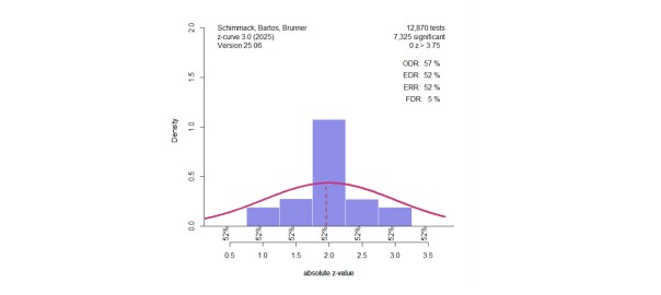
This chapter compares different transformations of t-values into z-values to be analyzed with z-curve. Only t-values are considered because F-values from studies with one experimenter degree of freedom can be converted into t-values, t = sqrt(F). Chi-square tests with one degree of freedom can be converted into z-scores, z = squrt(chi-square). Test-statistics with more complex designs are rare and do not test a clear hypothesis. They require follow up tests to determine the pattern and the follow-up tests can be used.
Chapter 8: From t-values to z-values
The t-distribution was discovered in 1908 by William Sealy Gosset, a statistician at the Guinness Brewery in Dublin. It is useful when the population standard deviation is not known, and sample sizes are small. Ronald A. Fisher later formalized its use within the framework of hypothesis testing and many comparisons of two groups or correlations rely on t-distribution for significance testing.
The problem for meta-analysis is that studies with different sample sizes have different distributions. A value of 2 is significant, p < .05, two-sided, with the normal distribution and in large sample sizes, but not in small sample sizes. Z-curve requires that all test-values are comparable and have the same sampling distributions. Therefore t-values need to be transformed into z-values. This approximation can introduce biases in z-curve results if sample sizes are small. The question is how big these biases are and how this bias can be minimized.
This blog post examines four methods to use t-values with z-curve.
1. The default method in z-curve is to use two-sided p-values and convert them into z-values. This approach is useful because it does not require information about the degrees of freedom.
2. Another approach that is often used in literatures with large sample sizes is to simply ignore the degrees of freedom and use the t-values as if they are z-values. z = t. The main problem of this approach is that t-values increasingly overestimate power as degrees of freedom decrease.
3. The third method is new and was developed for z-curve.3.0. Rather than computing the p-value under the null-hypothesis for all t-values, the method uses the mean of the t-values to pick the non-centrality parameter for the transformation. With low means, it uses a value of 0 and there is no difference to the p-value method. With moderate means, it uses a moderate non-centrality parameter around 2. For high means, it uses a high non-centrality parameter around 4. This changes the transformation distribution in accordance with the typical distribution of the observed t-values.
4. The fourth method uses the t-distribution to model the observed t-values. This method is essentially a z-curve with t-distributions and can be called t-curve. It is now implemented in z-curve 3.0 and can be used by supplying a fixed df value and requesting the estimation method “DF.” This method is useful when all studies have small df (N < 30), and because df cannot be less than 1, df of studies with small samples have a relatively small range with similar distributions.
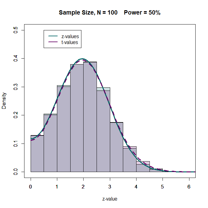
The illustration first shows the effect of degrees of freedom on the t-distribution when power is 50%. Figure 1 shows the results for studies with N = 100 (df = 98 for a two-group comparison). The distributions are not identical, but very similar and have little influence on z-curve estimates.
.
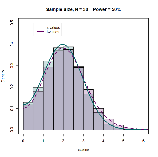
What happens when sample sizes are smaller. In the (not so good) old days, sample sizes were often n = 20 per group. This gives a total sample size of N = 40 and 38 degrees of freedom. However, sometimes some values are missing. Let us examine a scenario with N = 30. The distributions are still fairly similar. How do these small differences influence z-curve estimates?
The z-curve estimates for the z-values are within 1 percentage point of the true values.
The z-curve estimates based on the t-values are slightly inflated and the difference is 5 percentage points for the ERR. The results for other levels of power are similar (see simulation results below).
The next figure shows the results for t-values converted into p-values and then converting p-values into z-values. This procedure does not produce z-values and the distribution is slightly different than the distribution for actual z-values, but the transformation produces slightly better estimates than the use of t-values as z-values.
The next figure shows the results using conversion of t-values to power and then converting power to z-values. With a median of the significant t-values of 2.8, a value of 50% power is used for the transformation. This produces perfect estimates when power is indeed 50%. Some bias will be introduced when the power of the transformation does not match the true power. The extend of this bias will be examined in the simulation study. The illustration shows that using p-values or power is not identical because the t-distribution differs for different non-central t-values.
Finally, I added a t-curve option to z-curve.3.0. Users can provide a df-value and request fitting t-distributions with the specified df-value to the data. When all studies have the same df, the model fits perfectly.
The illustrations used all observed data, but z-curve was developed for datasets with selection bias. The simulations examine the performance of the different methods when only significant results can be used and z-curve estimates the average (unconditional) power of the studies with significant results (i.e., the expected replication rate, ERR), and extrapolates from this distribution to estimate the full distribution, including the missing non-significant results. The average power of all studies is the expected discovery rate (EDR) that predicts how many significant results researchers actually observed when they analyzed their data. When the EDR is lower than the observed discovery rate (i.e., the percentage of reported significant results), we have evidence of publication bias.
The Simulation
The setup of the simulation study is described in more detail in Chapter 4. The most important information is that the original studies are assumed to be mixtures of three normal distributions centered at 0, 2, and 4. To obtain t-values, the z–values are converted into power (loosely speaking, for 0 the value is 0 and H0 is true and power* is alpha). The power for z2 is 50% and the power for z4 is 98%. With weights ranging from 0 to 1 in 0.1 steps, we get 66 unique mixtures of the three components. The simulation simulates large sets of studies, k = 100,000 to minimize random sampling error and reveal systematic biases in the different estimation methods. The simulation uses only significant results to see the performance of the transformation methods when selection bias is present.
Results
Expected Replication Rate
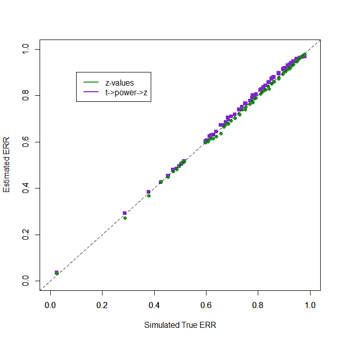
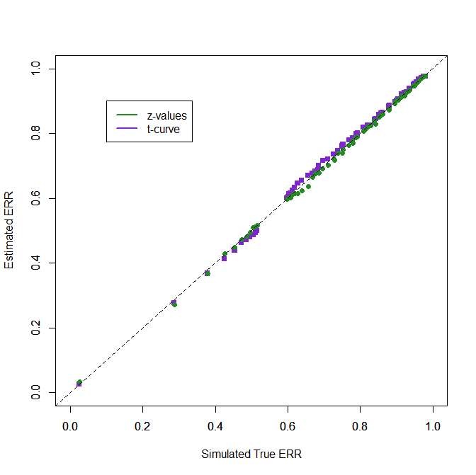
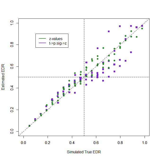
The expected replication rate is the average probability of studies with significant results to produce a significant result again in an exact replication study. To compare the estimates of the ERR, I computed the root mean square error (RMSE). A value of .01 implies that estimates are on average within 1 percentage point of the true value.
Method RMSE 1. z-values………….. .005 2. t-values …. ……… .081 3. t -> p -> z ..,,…….. .026 4. t -> power -> z…. .011 5. t-curve …………… .005
The results show that the use of t-values as if they were z-values is inferior to other methods. The default approach to convert t-values into p-values and the p-values into z-values works better, but the new methods work even better. Not surprisingly, analyzing t-values with 28 degrees of freedom with a model that fits this assumption works as well as analyzing normal distributions with z-curve that assumes normal distributions of sampling error.
The next figure examines the performance of the methods visually using the results for z-values as a standard of comparison.
1. Using t-values as z-values
2. Default transformation in z-curve 1.0 and 2.0
Using t-values as if they were z-values leads to overestimation of power because t-values are larger than z-values. More interesting is that the bias is more pronounced for lower levels of power. When the null-hypothesis is true, t-values estimate 20% power, a very misleading result.
The default method does not have this problem. It can identify sets of studies with only false positive results. It shows the opposite trend to underestimate power for moderate levels of power, but the bias is small and not practically relevant. It does well for moderate to high power and only shows a small trend to underestimate again close to the maximum probability of 1. Overall, these results show that the default transformation of t-values into z-values that has been used in published articles works reasonably well even if sample sizes are as small as N = 30. As most studies have larger samples sizes and bias is even smaller, the approximation of t-values with z-values does not undermine the validity of z-curve results. This confirms earlier findings with simulations that used t-values and typical sample sizes from psychology (Bartos & Schimmack, 2022; Brunner & Schimmack; 2020). Remember that these results also generalize to F-tests with 1-experimenter degree of freedom because these F-values are just squared t-values.
3. Transformation with (Unconditional) Power
However, some areas in psychology have even smaller sample sizes than N = 30, and the bias of the default method gets larger. In these situations, users of z-curve can use one of the two new methods. The first approach uses the probability of a significant result (loosely called power) to convert t-values into z-values. The probability is chosen based on the median t-value of the significant results. When it is low, a probability of 5% is used and the conversion is like the p-value conversion. When the median significant t-value is moderate, a probability of 50% is used and the non-central t-value and z-value that produce this probability is used. When the median significant t-value is high, a probability of 75% and the corresponding non-central z and t-values are used. The specific values are not relevant. What is important is that the t-distribution approximates the distribution of the true distributions better when the non-central values are closer to the actual ones. The figure shows that this method performs as well as z-curve analysis with true z-values for the full range of ERRs.
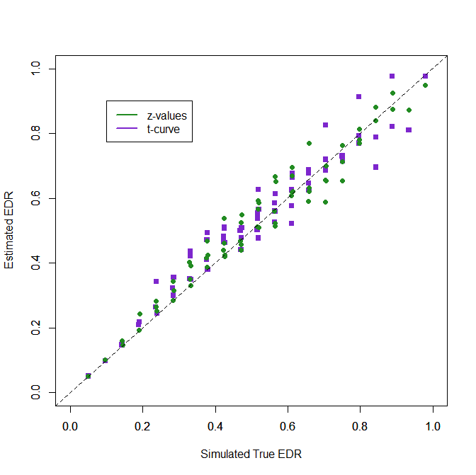
4. Analyzing t-values with t-curve
The t-curve option simply fits the mixture model of z-curve using t-distributions with a fixed df for all studies. It does as well as z-curve with z-values and does not require a conversion of test-statistics. Thus, it is the preferred method to estimate ERR for sets of studies with small df.
Expected Discovery Rate
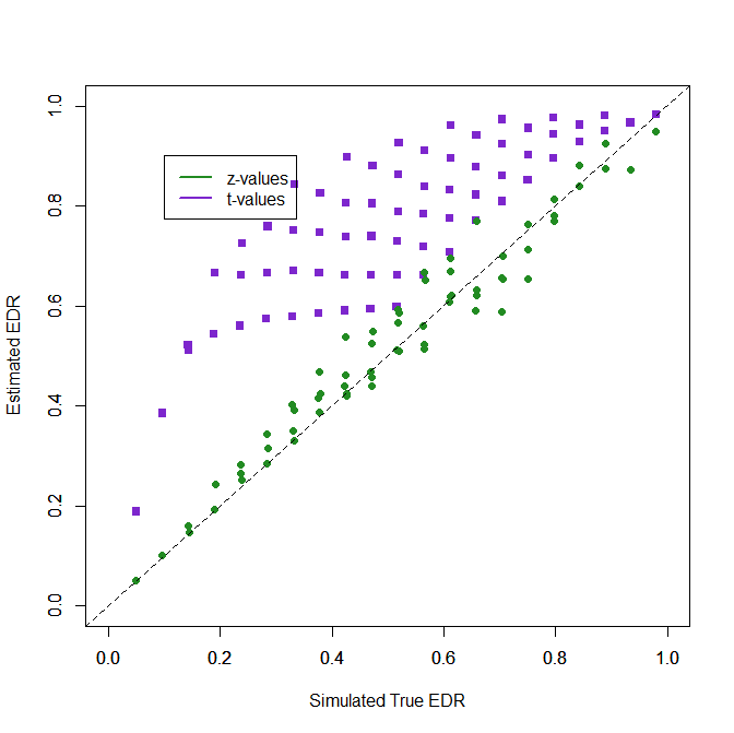
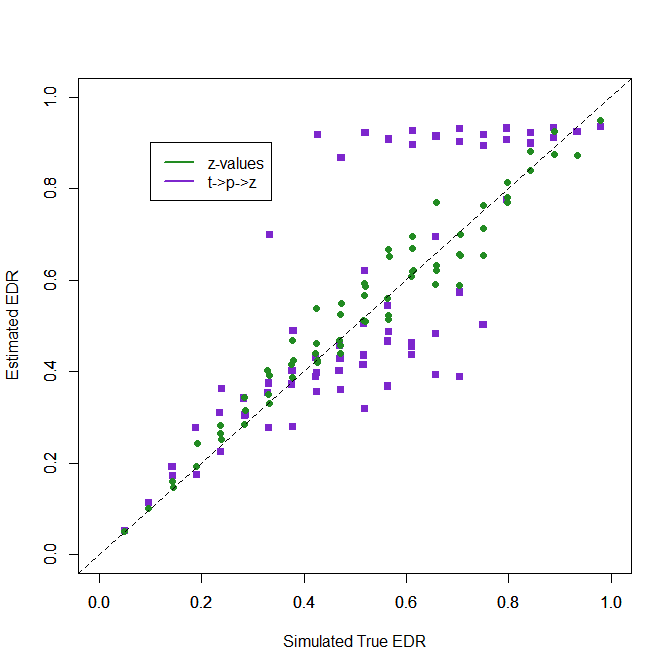
The expected discovery rate (ERR) is the average probability of all studies to produce a significant result, including studies with non-significant results. As non-significant results are not observed due to simulated publication bias, z-curve has to guess the distribution of non-significant results from the distribution of significant results. This leads to more uncertainty and more room for bias in EDR estimates and the RMSE values are larger than the RMSE values for the ERR. The question is only how transformation methods compare to the estimates based on z-values.
Method RMSE 1. z-values…………. .049 2. t-values … ……… .280 3. t -> p -> z ..,,……. .165 4. t -> power -> z…. .090 5. t-curve …………… .057
Three patterns in the RMSE results are noteworthy. First, the default transformation introduces considerable bias in the estimation of the EDR. Second, the new transformation using differnet levels of unconditional power is a notable improvement. Finally, analyzing t-values with t-curve also is notably better than using transformations. Why t-curve with t-values shows slightly worse fit than z-curve with z-values is not clear at this moment, but the difference is minor and using the t-curve option is recommended if all or most studies are small.
1. Using t-values as z-values
No comment.
2. Default transformation in z-curve 1.0 and 2.0
Some comments are required for the default method. First, the plot is ugly, but remember it is based on a sample size of 30. So, it merely shows that the default method should not be used when most studies are small which has not been the case in actual applications of z-curve to real data.
Second, the biggest problem is that z-curve overestimates the EDR when the true EDR is high. The reason is that it can be tricky to detect that the published studies with high power were obtained from also testing a large number of studies with low power that produce few significant results and are not “published.”
From a practical point of view, this is not a big problem. Say researchers conduct 4 small pilot studies with low power. They publish these pilot results when they produce a significant result, but do not report them when they do not. Then they conduct a more powerful study that is more likely to produce a significant result. Omitting the small pilot studies with non-significant results does not distort the literature. The real problem remains that the larger more powerful study is not reported if it also does not produce a significant result. This is revealed by the ERR. In real datasets, these patterns are rare and most z-curves show a mode (peak) at 1.96 rather than at 4.
3. Transformation with (Unconditional) Power
The new transformation using unconditional power works better because it does a better transformation for large t-values. The key problem that remains is that moderate ERRs in the 50-70% range are underestimated, but most true EDRs over 50% are estimated to be over 50%, and those below 50% are estimated to be below 50%. The transformation is used when most studies have larger sample sizes. So, the bias seen here is reduced by the percentage of studies with small sample sizes.
4. Analyzing t-values with t-curve
When all studies have small df, the new t-curve method can be used. The results for t-curve with t-values and z-values with z-curve are difficult to distinguish. There appears to be a bit more variability for really high values. Nevertheless, these results provide the first validation evidence for the use of t-curve. The good performance of t-curve is of course expected. All models work well when simulated data meet the assumptions of the model. Further validation research needs to examine how well t-curve works when small studies have different sample sizes. With really small df (df < 5) the method may not work well, but then, why not collect data from 3 more participants or just do a replication study with twice the sample size (N = 10)? (LOL).
Conclusion
Z-curve uses transformation to z-values to model sampling distributions of different statistical tests. This can introduce bias because sampling distributions of other tests differ from actual z-tests. Here I examined how much bias different transformations produce and presented a new transformation method that works better than the default method used in z-curve 1.0 and 2.0. I also showed that data from small samples can be better analyzed using actual t-distributions and demonstrated the performance of the new t-curve option. The results address concerns that z-curve estimates are not trustworthy because each test has a different sampling distribution. This broad criticism is not valid because differences between t-distributions and the standard normal are trivial once we reach even modest sample sizes of N = 100. Even for sample sizes of 30, the transformation introduces only small bias for the ERR and EDR estimates are still useful. Users of z-curve need to be aware of the possibility of bias, but they can be confident that z-curve produces useful estimates of (unconditional) power that can be used to estimate expected discovery and replication rates.
This blog post was co-authored by ChatGPT. I asked ChatGPT questions during the research for this post and ChatGPT wrote the draft. I verified the content and made some edits. I am fully responsible for the content of this post and all mistakes are my own. Happy to correct mistakes if you point them out in the comment section or an email.
Erratum: In an earlier post, I misattributed the definition of power as a conditional probability to Jacob Cohen. This was a mistake. I checked Cohen (1988) and found – much to my surprise and chagrin – that I had trusted ChatGPT too much. My mistake. Cohen actually writes.
I happily apologize to Cohen and to restore his reputation in my mind. His dedication and futile efforts to teach psychologists how to do better research remains a shining example. I regret that I never had a chance to meet him in person. In hindsight, it makes perfect sense that lesser minds introduced the conditioning on a true effect (why? because psychologists are never wrong?) that led to ridiculous claims about power by Pek et al. (2024) in a journal for psychology methodologists (apparently an oxymoron). Pek et al. claimed that Cohen never meant for power analysis to be used to evaluate completed studies. Even this is a lie.
So much for the credibility revolution in psychology. Credibility requires expertise and proper citation of experts. I don’t see much of that in the “psycho – sciences.”
100 Years of Statistical Power: A Long and Confusing History
Neyman’s Type II error Jerzy Neyman introduced the importance of thinking about the probability of obtaining an undesirable non-significant result when the alternative hypothesis is true. He called this the Type II error.
Power curves and the null point Neyman provided researchers with curves and tables showing the probability of a Type II error for different effect sizes.
These included a value of zero effect size, which yields a probability of a non-significant result equal to 1−α. This is not a Type II error—because the null is true—but simply the probability of a non-significant result under the null.
The term “power” Neyman and Pearson also used the term power for the complement of the probability of a non-significant result. The corresponding probability of a significant result under the null is α. In other words, Power=1−P(non-significant result) or simply Power = P(significant result).
Implication for meta-analysis This original definition of power makes it straightforward to talk about the average power of a set of studies in meta-analysis. Even if some studies have true effect sizes of zero, the power values can be averaged to predict the overall percentage of significant results—what Bartos & Schimmack (2020) call the expected discovery rate. It is also possible to estimate the average power conditioning on significance by taking selection bias into account (Brunner & Schimmack, 2020), even if some of the significant results are false positive results with a true effect size of zero.
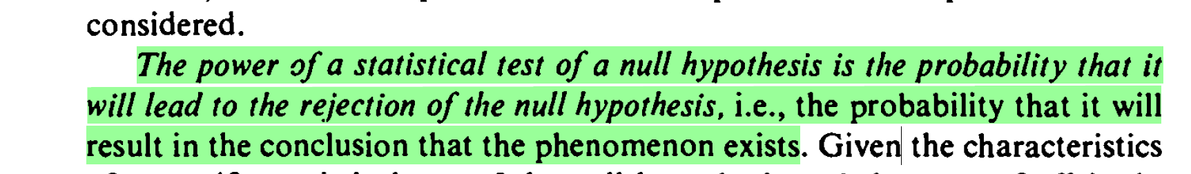
Cohen’s Influential Work on Power Jacob Cohen popularized the concept of power in the social sciences, especially psychology. He followed Neyman’s definition of power and defined it as follows. “The power of a statistical test of a null hypothesis is the probability that it will lead to the rejection of the null hypothesis, i.e., the probability that it will result in the conclusion that the phenomenon exists” (p. 2). This definition implies that power is also defined when the null-hypothesis is true and a significant result is a false positive result. The probability in this case is easy to compute. Power = alpha, ween H0 is true.
Psychologists Redefine Power However, psychologists started to redefine power (a history that still needs to be researched). Nowadays many textbooks and articles by psychologists define power as a conditional probability that assumes an effect size different from zero (H0 is false, H1 is true). Many psychologists falsely belief that this was always the definition of power (including myself until I did this research). This definition made sense for planning studies, but it is less suited for describing completed studies, because in reality, the true effect size could be zero.
Cohen’s assumption about true effects Cohen may also not have thought that it is important to distinguish between the probability of a significant result and the conditional probability of a significant result if the null hypothesis is false. He made fun of the nil-hypothesis as a serious hypothesis (The Earth is round, p < .05) and assumed that most studies have non-zero effect sizes. So, the distinction between conditional and unconditional probabilities is practically irrelevant.
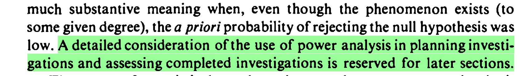
The resulting confusion The definition of power as a conditional probability, however, led many psychologists to adopt a restricted view of power. Some now argue (e.g., Pek et al., 2024) that power is only meaningful as a pre-study, hypothetical quantity based on assumed non-zero effects. In contrast, Cohen clearly considered the use of power to evaluate completed studies. “They can also be performed on completed studies to determine the power which a statistical test had” (p. 14). Pek et al. (2014) use the new definition of power as conditional on a true effect to argue that this is not possible to apply power to completed studies. The use of power “as a criterion to evaluate the credibility of results from completed research, conflicts with definitional properties of statistical power.” (p. 2). This is true, but only if we define power as a conditional probability, which is not the original meaning of the term. Pek et al. are not alone in their confusion about power. In an article that aims to dispel myths about power on a blog post by the American Psychological Society (renamed as Association for Psychological Science), Lengersdorff and Lamm (2025) use the conditional definition of power as “the probability with which a statistical test will produce a significant result, under the assumption that the tested effect exists” They then make the false claim that “it depends on the expected effect size” This has nothing to do with the actual probability of getting a significant result that depends on the true population effect size. It gets worse from there on. With self-proclaimed experts who cannot even quote Cohen correctly, psychology is doomed to remain the science with important questions and no answers. ,
Resolving the confusion We can resolve the confusion in two ways. Either we reeducate psychologists about the definition of power as the unconditional probability of a statistically significant result in an actual study that depends on the actual size of the effect, if it could be observed without sampling error or we concede that this is a futile battle and simply find a new term for this important probability that can be used to evaluate the p-values that psychological scientists use to claim that they discovered some fundamental laws of human nature. We could call it, Probability of Statistical Significance (POSS). Studies with high POSS are more credible than studies with low POSS, especially when the studies with low POSS surprisingly always have significant results. Everything psychologists’ power cannot do, POSS can do.
My Personal Preference My preference is clear. Cohen has done a lot to popularize power among social scientists, and his 1988 book remains the foundational book on this topic. The book clearly defines power as the probability to obtain a significant result. If psychologists are not able to read, it is their problem and not the problem of those who actually understand statistics. If they want to remain ignorant and do not want to evaluate the power of their studies, so be it. Others will and if the results are not good, they may lose funding. Cohen (1988) predicted that psychologists will ignore power “at their peril.” Well, they were able to survive with power for another 40 decades, but maybe Cohen’s prophecy is coming finally true. All their attempts to avoid facing the music are futile. The use of power to evaluate their published p-values is like using modern doping test to detect doping in frozen urine samples from 1960. We can tell, which p-values were obtained with high POSS, which ones were not, building on Neyman, Pearson, and Cohen.
Epilogue(Personal Reflection) I Jerry (Brunner) and I are big fans of Cohen and without his work, we would not have developed z-curve; a tool that can estimate average power. I was happy to learn (after I first attributed the mistake to Cohen) that he correctly stated the definition of power as the probability to obtain a significant result, in accordance with Neyman. Psychologists then messed it up and are now fighting the use of power to evaluate their studies (Pek et al., 2024; ), Lengersdorff and Lamm (2025). Cohen clearly stated that we can use power to evaluate study outcomes. It remains a mystery to me why Cohen never tried to estimate the true power of studies to make a stronger case for the need of power analysis in psychology. It was only in the early 2010s that I started doing so and discovered the power of statistical power to reveal publication bias in multiple study articles (Schimmack, 2012). This work and the work on z-curve with my colleague follows directly from Neyman-Pearson’s influential work nearly 100 years ago. Neyman is the GOAT of statistics (he also created confidence intervals that make Fisher’s p-values useless). Although APA now recommends confidence intervals, too many psychologists still focus on p-values and do not understand that power determines whether their confidence intervals include zero or not. Statistics training would be easier and better if we got rid of Fisher, who was also a racist and eugenicist into the 1950s. Others before me have complained about the mindless use of statistics in psychology (Gigerenzer, 2004), but that has not changed practices. Maybe the time has come. Let’s build our statistics training on solid foundations. Fisher is dead. Long live Neyman and the definition of power as the probability to get a significant result in an actual study that depends on the true population effect size.
I have posted several blog posts about Pek et al.’s (2024) flawed discussion of power as a tool to evaluate published studies. Some readers have questioned my interpretation of the article. “Surely, this is not what they are saying.” Indeed, their claims are so ridiculous that it is hard to believe that a respected journal published the article. To make clear that they are saying exactly what I am saying they are saying (oh boy), I found relevant quotes and asked ChatGPT to translate them to avoid my own biases in the interpretation of their writing. ChatGPT also provided a point by point comparison of their key claims and my rebuttal.
I sent Pek this summary to check whether this summary of her position is accurate. I will let you know if there is a response. Feel free to express your own views in the comments section.
1. Core Claim #1 — Power is a Pre-Data Property, Not a Post-Data Measure
Plain language: They argue that statistical power is defined as the probability of rejecting H0H_0 before you see the data, given a specified α\alpha, effect size, and sample size. Once the study is completed and the data are fixed, that probability no longer applies — you can’t “retroactively” assign a probability to an event that has already happened.
Quote:
“Thus, power is a property of a test (procedure) for some value of α, N, and μ and not a property of observed data.” (p. 7)
Quote:
“Applying a probability over random data to fixed (observed) data is a fatal ontological error.” (p. 8)
2. Core Claim #2 — Using Observed Power is Mathematically Redundant with the p-value
Plain language: If you calculate “observed power” from the observed effect size and sample size, you are just transforming the p-value into another scale. This means observed power adds no new information beyond what you already get from the p-value.
Quote:
“Because observed power is a transformation of the p-value, it provides information about the completed study that is mathematically redundant with the p-value.” (p. 6)
3. Core Claim #3 — Using Power to Evaluate Completed Studies Is Counterproductive
Plain language: They argue that using power as a “credibility check” for published research can be misleading and harmful. They frame this as “power for evaluation,” meaning applying power calculations to completed studies to make judgments about them (either singly or in aggregate). They say this conflicts with the definition of power and encourages the misuse of probability for fixed outcomes.
Quote:
“We also describe why using power for evaluating completed studies can be counterproductive.” (Abstract)
Quote:
“Power for evaluation…conflicts with definitional properties of statistical power and should be discouraged.” (p. 5)
4. Core Claim #4 — Average Power Estimates Still Inherit the Same Problems
Plain language: Even if you aggregate many studies and calculate “average observed power” from meta-analytic effect sizes or benchmarks (e.g., Cohen’s “t-shirt” effect sizes), you’re still plugging in effect size estimates from data. They say this is just a more complicated version of the same post-hoc problem — the estimate is imprecise, biased, and conceptually inappropriate for evaluating completed studies.
Quote:
“Analytical and simulation evidence…demonstrates that average observed power is relatively uninformative because its estimate is highly variable and imprecise…using observed power calculations to make statements about the power of tests in those completed studies is problematic because such an application of power is an ontological impossibility of frequentist probability.” (p. 13)
5. Core Claim #5 — Estimates Based on “T-Shirt” Effect Sizes Are Especially Unreliable
Plain language: When researchers take a benchmark effect size (e.g., “medium = 0.5”) and combine it with the actual sample sizes in published studies to estimate “average power,” Pek et al. say this is disconnected from the actual effects in the literature. They argue that these benchmarks are hypothetical and therefore do not reflect the true power of the completed studies.
Quote:
“Taken together, power calculated from hypothetical t-shirt effect sizes μ and N̂ cannot be deemed to reasonably reflect the power of completed studies.” (p. 12)
6. Supporting Argument — Appeal to Authority & Prior Warnings
Plain language: They cite multiple influential statisticians and methodologists who have criticized post-hoc power. This is meant to reinforce that the problems they’re pointing to are widely recognized, not their invention.
Quote:
“…unsurprisingly, this ontological error has prompted several influential statisticians and methodologists to object to poststudy applications of power.” (p. 9)
7. Supporting Argument — Power Calculations Should Be Reserved for Planning Future Studies
Plain language: Their preferred framing is that power is for design, not evaluation. They suggest that if you want to assess completed research, you should use other tools (though they don’t strongly recommend specific alternatives).
Quote:
“Uses of Uncertain Statistical Power: Designing Future Studies, Not Evaluating Completed Studies” (title)
“We emphasize that the most useful role for power is in designing studies, not in evaluating completed research.” (paraphrased from discussion)
Pek et al. vs. Rebuttal — Point-by-Point
Pek et al. Claim / Quote
Rebuttal
Power is a property of a test (α, N, μ) and not a property of observed data“Applying a probability over random data to fixed (observed) data is a fatal ontological error.”
Power is indeed defined for the population parameters, but we routinely estimate unknown population parameters from data. Estimating μ from observed data and then computing power from it is no more an “ontological error” than estimating μ itself. Both are subject to sampling error but not conceptually invalid.
Observed power is a transformation of the p-value and adds no new information
True for a single study without bias correction, but irrelevant when aggregating many studies, modeling publication bias, or estimating the power distribution. In z-curve, p-values are used collectively to estimate the underlying distribution of true effects and selection, which yields information about replicability that is not in any single p-value.
Power for evaluation is counterproductive and should be discouraged
This overgeneralizes from the misuse of single-study observed power. Field-level evaluations (e.g., z-curve, excess significance tests, BUCSS) use many studies and account for bias, providing valuable diagnostics of research credibility. Discouraging this removes a key tool for detecting systemic issues.
Average observed power from meta-analytic effect sizes is imprecise, biased, and conceptually inappropriate for completed studies
All statistical estimates are uncertain — precision improves with larger datasets. Meta-analytic average power, especially when bias-corrected, is an interpretable measure of expected replicability. Critiquing its imprecision without considering dataset size or bias correction ignores advances like z-curve that address these limitations.
“T-shirt” effect sizes (e.g., Cohen’s benchmarks) do not reflect actual effects in the literature
Benchmarks are crude, but many “low power in psychology” studies use empirically derived effect sizes from actual published results — not just hypothetical 0.2/0.5/0.8. Even if initial estimates are imperfect, they provide a baseline showing the mismatch between typical sample sizes and plausible effect sizes.
Appeal to authority: influential statisticians warn against post-hoc power
Most of these warnings target naïve single-study calculations, not sophisticated bias-corrected meta-analytic methods. Citing these warnings to dismiss all uses of power for evaluation is a straw man.
Power should be reserved for study planning, not evaluating completed research
Evaluation is essential for identifying systemic underpowering and bias. Without it, we cannot quantify the gap between claimed and actual evidential value in a literature. Tools like z-curve and BUCSS bridge the gap between evaluation and design by using completed studies to inform better future research.
Footnote on Brunner & Schimmack (2020) and Simonsohn et al. (2014): labeling average power a “replicability estimate” is misleading
This criticism ignores that average bias-corrected power does correspond to the expected proportion of significant replications under similar conditions — which is the definition of replicability in this context. The label is appropriate when the estimation method accounts for selection and heterogeneity, as in z-curve.
Psychologists are not famous for their quantitative chops. Many undergraduate students treat statistics courses as an ordeal to survive, not a skill to master. In North America especially, large psychology departments rely on large undergraduate programs for funding, which creates pressure to keep students happy. One way to do that is to offer “statistics-light” courses that avoid scaring off tuition-paying customers. As a result, most psychology majors graduate believing that the key to scientific discovery is to get p-values below .05, and that the results in their textbooks are trustworthy simply because they are “statistically significant.”
Graduate Training Isn’t Much Better
The situation doesn’t improve much in graduate school. Students learn how to point-and-click their way through statistical software, run analyses, and search for p-values below .05—this time with the added incentive that significant results mean publications for them and their advisors.
Over sixty years ago, Sterling (1959) warned that this obsession with p < .05 undermines the already limited value of p-values. Cohen (1994) memorably satirized the mindset with his title “The Earth is Round, p < .05.”
Sterling (1995) also documented a glaring oddity: psychology papers overwhelmingly report significant results—often 90% or more. That kind of hit rate would require researchers to be right almost all the time in their predictions. Given that most psychologists use two-sided tests (“Does X increase or decrease Y?”), they can claim a “hit” in either direction. The only way to be wrong is if the true effect is exactly zero—something many argue is rare.
But there’s another reason to be skeptical: to produce so many p < .05 results without fraud or extreme data-torturing, studies would need high statistical power. And here’s the rub—psychologists’ understanding of power is notoriously shaky. Even some quantitative psychologists, who should know better, end up publishing articles that confuse rather than clarify (see Pek et al., 2024).
What Power Actually Means
I’ve taught undergraduates about statistical power for over a decade, and AI can now spit out perfectly serviceable definitions in seconds. Here’s one example:
Statistical power is the probability that a statistical test will correctly reject the null hypothesis (H₀) when a specific alternative hypothesis (H₁) is true—in other words, the probability of detecting an effect if it exists. Power = 1 − β, where β is the Type II error rate.
Power depends on: Effect size (true magnitude of the effect) Sample size (bigger samples, higher power) Significance level α (threshold for rejecting H₀) Variability (less noise, more power)
Power is Unknown
Why care? High power reduces false negatives, makes non-significant results interpretable, supports replicability, and prevents waste of resources. Most important, power helps researchers to get the desirable p-values below .05. Why would you not plan studies to have a high probability to get a significant result, as long as the effect is not really zero.
The problem is that power depends on the the true(population) effect size. We never actually know this value—we only estimate it from samples, and those estimates vary because of sampling error. This uncertainty is not a special flaw in power analysis; it’s the nature of empirical research.
When planning studies, researchers must guess effect sizes, plug them into a formula, and get a required sample size—often aiming for the conventional 80% power. In practice, that number often comes from convenience (“How many participants can we realistically get?”) rather than a solid prior estimate and sometimes power analysis are fudged to put in a sample size and get the effect size that would give 80% power.
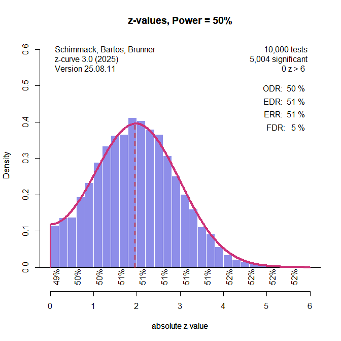
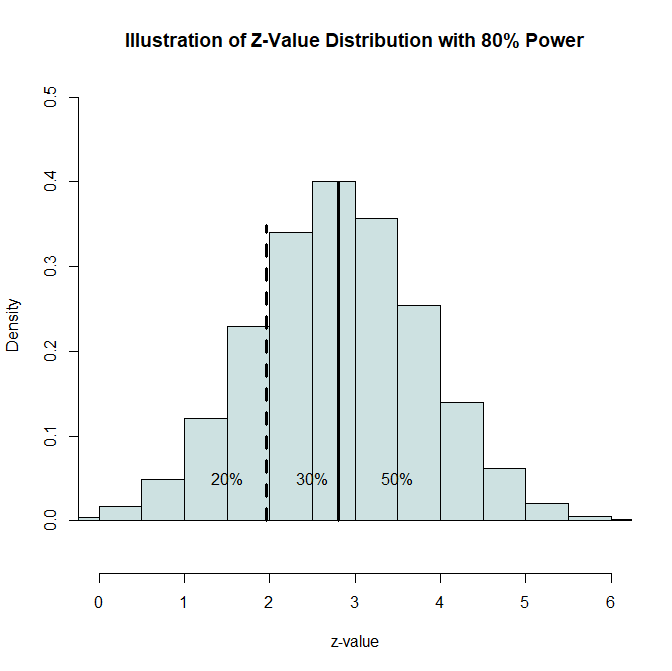
What 80% Power Looks Like
If we truly designed studies with 80% power and guessed the effect size perfectly, the resulting test statistics (converted to z-values) would form a predictable distribution:
Figure 1. Distribution of z-values with 80% power. The dashed line marks the significance threshold (z = 1.96, p = .05), and the solid line marks the expected mean z for 80% power (z ≈ 2.8).
20% fall below the significance cut-off (non-significant)
30% are significant but below the expected mean
50% exceed the expected mean
This breakdown is a theoretical benchmark. If actual published results deviate strongly from it—say, 90% significant results instead of 80%—we know that our hypothesis that all studies have 80% power is wrong. Either researchers consistently underestimated effect sizes (unlikely), or results were selectively reported to favor significance (more likely).
Why Pek et al. Are Wrong About “Only for Planning”
Pek et al. (2024) argue that power is fine for planning studies but should not be used to evaluate completed ones. This is like saying we can predict a distribution under the null hypothesis and use it to interpret p-values, but once we see our data, that prediction magically disappears. It doesn’t. It is actually needed to draw inferences from the observed p-values. Thus, we are comparing actual data to a hypothetical distribution to make inferences about the direction of an effect.
The same is true for hypotheses about power. If we assume 80% power, we can predict the shape of the sampling distribution (Figure 1) and compare it with actual published data. Deviations tell us whether the true power was likely higher, lower, or compromised by selective reporting.
A Simple Example
Consider Wegener & Petty (1996), Study 2, which had three independent samples. The key interaction effect produced z-values of 2.03, 1.99, and 2.53. All are significant but fall between 1.96 and 2.8.
With 80% power, there’s only about a 30% chance of landing in this range in a single study. Doing so three times in a row has a probability of about 0.027—well below the usual 0.05 cut-off. This suggests the results were not from well-powered studies that got lucky to produce 100% significant results with 80% power, but more consistent with low power plus selective significance.
The Real Value of Power
Ironically, power is not that useful for planning studies—because effect sizes are unknown and easily fudged. Its real strength is as a diagnostic tool for evaluating the credibility of published results. If the distribution of test statistics doesn’t match what we’d expect from a plausible power level, we have reason to doubt the findings.
This doesn’t require knowing the exact “true” power—just as we can test the null hypothesis without already knowing the population effect size. Similarly, we can make predictions based on hypotheses about power and use them to evaluate observed data. It just does not follow, that we can draw inferences from normal distributions at 0, but not from normal distributions centered at 2.8 or some other value, but many psychologists confuse null-hypthesis testing with nil-hypothesis testing (Cohen, 1994).
Final Thoughts
The resistance to using power this way is puzzling. Maybe it’s a misunderstanding of the concept, maybe it’s a desire to shield the literature from uncomfortable scrutiny. Either way, learning about power is not just a technical exercise—it’s a tool for scientific self-defense. If you see a literature where most p-values cluster between .05 and .005, be skeptical. If they’re mostly below .005, you can have more confidence.
Understanding power gives you the ability to look beyond “statistically significant” and ask: Was this result ever likely to be true?
Cookie Consent
We use cookies to improve your experience on our site. By using our site, you consent to cookies.