First, a sigh of relief. We made it through 2025, despite the rise of evil in the world. Let’s all hope or pray that 2026 will be better. In our little and mostly harmless world of psychology, however, things were rather calm. Here are some stats from my blog post to review 2025.
Clicks and Engagement
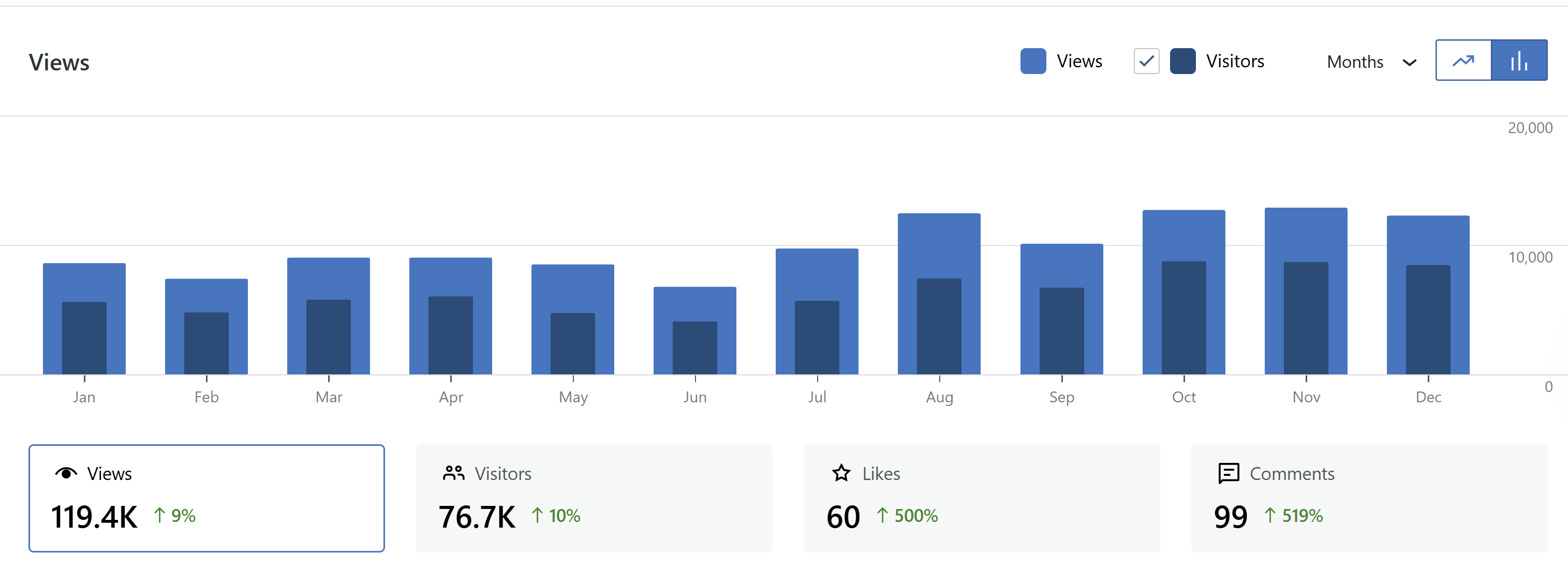
Many of these stats are bots and 1second visits, but some are real humans who are interested in scientific psychology and how to make it better. As long as I see these levels of engagement, I feel encouraged to keep the blog going. Likes and comments are rare, but very much appreciated. As the saying goes, one comment is worth more than 1,000 visits.
Content
The posts about “Fast and Slow” are still the most viewed pages. Reconstruction of a train wreck is home to Kahneman’s humble response to the z-curve analysis of the priming chapter, but the “Meta-Scientific Perspective” post is a review of all chapters.
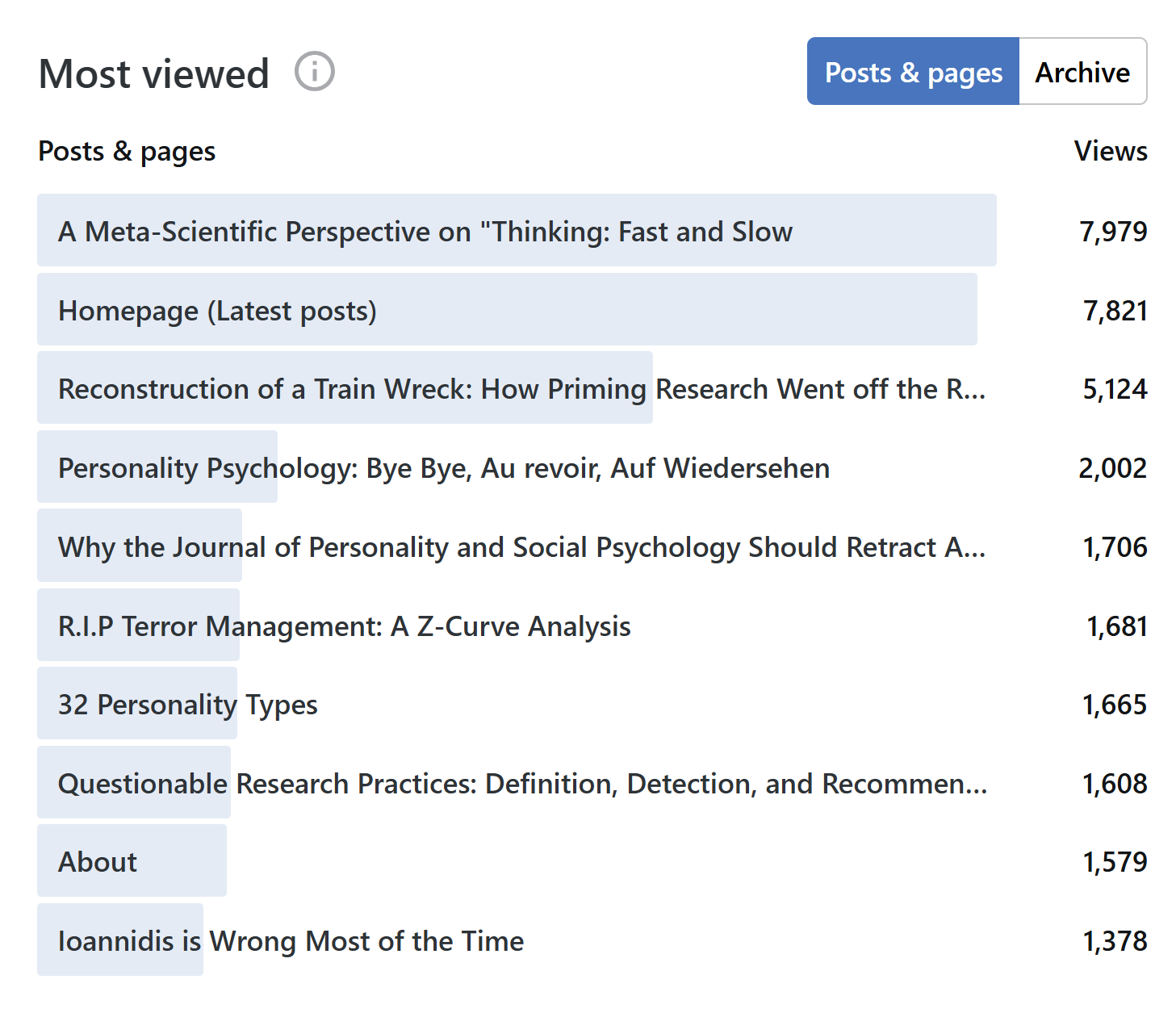
The surprising addition is my farewell to personality psychology. It was an emotional rant expressing my frustration with bad measurement practices and unwillingness to improve them in the field.
Personality Psychology: Bye Bye, Au revoir, Auf Wiedersehen – Replicability-Index
I was ready to give up on it entirely, but ironically, I am still teaching an undergraduate course on personality, which I define as the study of personality differences. Fortunately, there is enough research and open data that I can analyze myself that I can teach the course form a coherent scientific perspective. The textbook is now available on the blog.
Personality Science: The Science of Human Diversity – Replicability-Index
Another surprise is that the new post on terror management made the Top 10 list. I thank the author for including z-curve in their meta-analysis. The article shows that an entire literature with more than 800 studies can be made up of studies with low replicability and a high false positive risk. It also shows how z-curve is superior to p-curve that can only reject the null hypothesis that all (100%) of the studies are false positives, but not that 95% are.
R.I.P Terror Management: A Z-Curve Analysis – Replicability-Index
Below the Top 10 are still some noteworthy posts from 2025.
Why Uri Simonsohn is a Jerk – Replicability-Index (967 views)
I found an old email that referred to Uri as a jerk. The complaint was that the datacolada team are all about open science and criticism of others, but do not even allow people who are criticized to post an open response on their blog. No comments, please! I say that is not open science. That is just like legacy journals that do not publish comments they do not like (yes, I mean you Psychological Methods).
Review of “On the Poor Statistical Properties of the P-Curve Meta-Analytic Procedure” – Replicability-Index (657 views)
A related post features a critique of p-curve that later triggered a “no comments allowed” response by Uri on the datacolada blog. After 10 years of p-curve, it is fair to say that it has only produced one notable finding. Most of the time, p-curve shows evidential value; that is, we can reject the null hypothesis that all results are false positives. So, concerns about massive p-hacking in the false positive article are not empirically supported. The area of false positive paranoia is coming to an end. More on this, in a forthcoming post.
The Ideology versus the Science of Evolved Sex Differences – Replicability-Index (649 views)
My personality textbook includes a scientific review of the research on sex-differences. It debunks many stereotypes that are often dressed up as pseudo-scientific evolutionary wet dreams of sexist pseudo-scientists like Roy F. Baumeister, who still is treated by some psychologist as an eminent scholar. To be a science, psychology has to hold psychologists accountable to scientific standards. Otherwise, it is just a cult.
Psychologists really confuse academic freedom with “you can say the stupidest things”, like one article that compared use of AI to dishonest research practices.
Is Using AI in Science Really “Research Misconduct”? A Response to Guest & van Rooij – Replicability-Index (649 views)
Many of these articles could be published as blog posts, saving us (tax payers) money.
Traffic
Most of the traffic still comes from search engines and over 90% of this traffic comes from Google. Next is Facebook, where I maintain the Psychological Methods Discussion Group.
The group was very active during the Replication Crisis times, but little discussion occurs these days. I would love to move it somewhere else, but I have not found an easy and cheap alternative. Interestingly, Open Science advocates also do not seem to see value in hosting an open forum for discussion. I tried to post on APS, but you have to pay to correct their misinformation. So, there you have it. Psychology lacks an open discussion forum (OSF); talk about scientific utopia. I left fascist X a long time ago, but still get traffic from there. I am now posting on Bluesky with little direct engagement, but apparently some people notice the posts and visit.

Most interesting are the visits from ChatGPT. I am fully aware of the ecological problems, but AI will fix many of the problems that psychology faces, and equally environmentally problematic conferences serve more the purpose of taxpayer-paid vacations than advancing science. Nothing wrong with perks for underpaid academics, but let’s not pretend it advances science when talks are just sales pitches for the latest pseudo-innovation. Anyhow, blogging is now more important than publishing in costly peer-reviewed journals because AI does not care about peer-review and is blocked from work behind paywalls.
Some academics rail against AI, but appearently they never used one. ChatGPT constantly finds errors in my drafts and helps me to correct them before I post them. It also finds plenty of mistakes in published articles and we often have a chuckle that this stuff passed human peer review. On that note, human peer-review sucks and can be easily replaced with AI reviews. At least you don’t have to wait months to get some incoherent nonsensical reviews that only show lack of expertise by the reviewers.
The traffic from ChatGPT also underestimates the importance of AI. Few people actually click on links to check information, but ChatGPT’s answer is still influenced by my content. Ultimately, the real criterion for impact will be how much our work influences AI answers.
Location
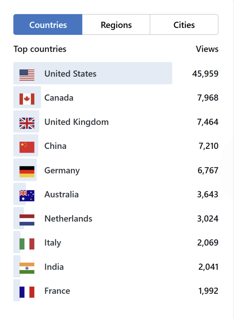
The United States continues to dominate psychology. Europe has more people, but only a few European countries invest (waste?) money on psychology. A clear North-West vs the rest difference is visible. Former communist East is just poor, but the problem in the South is religion.
One of the highlights of 2025 was my visit of the Winter school in Padua, one of the oldest universities. I learned that it was relatively free and Galileo made important discoveries there, but he ran into “a little problem” when he moved to Florence and clashed with the Catholic church. The lesson is that the broader culture influences science and currently the USA is showing that its values are inconsistent with science. Religious fundamentalism in the Confederate states is incompatible with science, especially a social one. China is on the rise, and it seems more likely that they will be the next home of psychology, unless Europe gets its act together. China is a totalitarian regime, but a communist dictatorship seems better than religious ones for science and for the future of the planet.
Forecast 2026
The main prediction is that traffic from ChatGPT and China will increase. Possibly, traffic from other AIs like Gemini will also emerge. Other developments are harder to predict and that is the fun of blogging. I don’t have to invest months of my limited remaining life span to fight stupid reviewers to be allowed to pay $3,000 or more of Canadian tax-payers money to share my work with the world. I can do so for free and just see whether somebody found the work interesting. Fortunately, I am paid well enough so that I do not have to worry about the incentive structure in academia that everybody knows leads to fast, cheap, and bad science, but nobody is able to change. For those of you who are still a cog in this mindless machine, I can say there is hope. The tyranny of publication cartels is weakening and maybe sometimes it is better to just post a preprint than to try the 10th journal for the stamp of approval in a peer-reviewed (predatory) journal. Academia is a long game. The rewards come at the end when you can do what you want without concerns about approval. Humanist psychologists call this self-actualization. I call it the freedom of not giving a fuck anymore.
See you in 2026,
Ulrich Schimmack
Happy New Year