You can find links to the other chapters on the post with Chapter 1.

Chapter 4 examines simulation studies to evaluate z-curve.3.0. zcurve3.0/Tutorial.R.Script.Chapter4.R at main · UlrichSchimmack/zcurve3.0

Introduction to Chapter 4

I assume that you are familiar with z-curve, but you may wonder how well it works. Nowadays it is easy to get information using a search of the internet. AI makes it even easier, but it also uses a lot of resources. Here is a summary of the current collective knowledge about z-curve’s performance.

“Z‑curve has been validated through numerous simulation studies—often more extensive than what’s published—and shows high accuracy and better bias control than p‑curve when studies differ in power or effect size. Confidence intervals generally maintain coverage. In real-world replication datasets, z‑curve predictions align closely with observed replication rates—better than p‑curve. Its performance is weaker only in extreme conditions with small or very homogeneous study sets.”

The problem is that this knowledge is based on simulation studies conducted by us, the developers of z-curve (Bartos, Brunner, & Schimmack). Maybe we hacked our simulations to show good performance and hide cases with bad performance. Yes, simulation hacking is a think. The question is: did we hack our simulations?

Science is not built on trust. it is built on trustworthy evidence from independent replications. This is difficult for empirical studies, but it is easy to do for simulation studies. If you run the same code with a seed, you are merely reproducing the published results because you generate the same random data with the same sampling bias. However, if you use a different seed (or no seed), you are replicating the results with a new roll of the dice. With large samples, the difference is negligible because sampling error is small. This tutorial allows you to reproduce or replicate simulations of z-curve to see for yourself how well or poorly it performs.

The Simulation

This tutorial uses the most basic simulation of z-value distributions with normal distributions with a standard deviation of 1. This assumes that tests are z-tests and that the tests fulfil the assumption of normally distributed sampling error. This is the ideal setting for z-curve. If tests’ assumptions are violated or other tests are converted into z-values, the performance may suffer. This is a topic for another chapter that focusses on the transformation of test results into z-values.

The simulation assumes that there are three sets of z-tests. Some test a true nil hypothesis. Tis is the standard normal distribution centered at zero. With alpha = .05, these studies have an unconditional power of 5%. That is, they have a 5% probability to produce a (false) significant result. The second set has moderate power. A z-value of 2 is practically right at the criterion for significance with a two-sided z-test, z = 1.96. This means that sampling error will produce significant results and non-significant results about equally. In other words, the test has about 50% power. Finally, z-values of 4 have very high power. The reason is that a normal distribution centered at 4 has only 2.5% values below 2, which is the significance criterion. So, power is about 97.5%.

To simulate different z-curves, the three distributions are combined with different weights ranging from 0 to 1 in steps of .1. You can change that to larger or smaller steps. This produces 66 unique combinations of the three components.

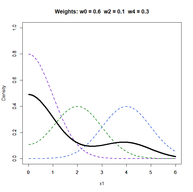
Figure 1 shows the folded density distributions of the three components and the density of the mixture distribution with weights 0.6 for the z0 component, 0.1, for the z2 component, and 0.3 for the z4 component. You can create your own mixtures to see the different shapes of z-curves. Broadly speaking z-curves that decrease have a strong weight on the z0 component and low average power and z-curves that increase have a high weight on the z4 component and high average power.

The simulation program samples from the three distributions. To examine systematic biases, the simulation created 50,000 z-values. You can change this, but then the performance is a function of systematic bias and sampling error. The performance in smaller and more realistic sample sizes will be examined in the evaluation of the confidence intervals provided by z-curve.

Z-curve uses two methods to fit the model to the data. The first method developed by Brunner and Schimmack first fits a Kernel Density model to the z-curve of the significant results (z > 2). Then the model is fitted to the Kernel Density distribution. The key problem with this model is that Kernel Density has a downward bias when values are truncated at 2. To avoid this bias, the curve is extended while taking the slope around 2 into account. The technical details are not so important. This method is fast and works well for the estimation of the Expected Replication Rate. However, the expected discovery rate projects the distribution for significant results into the region of non-significant results. Here even small biases around z = 2 can have large effects on the estimates.

The second method was developed by Bartos and Schimmack for zcurve.2.0. It uses the Expectancy Maximization method that directly fits all of the data points to the model. This method tends to work better for the EDR in some cases. The main drawback is that it can be slow when a large number of z-values are fitted to the model. For this reason, I prefer to use the old-fashioned, density method to explore the data and use the EM algorithm for the final results. The simulation here compares the results for both methods.

That is the same data are analyzed with both methods. To spare you time, I also provide the saved data from this simulation study.

Results

Expected Replication Rate

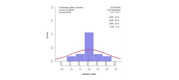
Each simulation keeps non-significant and significant results, but the model is only fitted to the significant results. Keeping the non-significant results helps to evaluate the ability of z-curve to predict the distribution of the non-significant results. This is illustrated in Figure 2.

Simulation #52 has the weights 0.6 for z0, 0.0 for z2, and 0.4 for z4. The true EDR is 43% and the true ERR is 91%. The observed discovery rate is the percentage of significant results in 50,000 tests. It is close to the expected value of 43%. Visual inspection shows that z-curve guessed the distribution of non-significant results rather well with a slight tend to underestimate non-significant results. This leads to a slight overestimation of the EDR by 1 percentage point. The model also correctly estimates the true ERR of 91%.

Of course, I am showing you an example that works well. So, don’t trust the picture. Trust, the results of all 66 simulations or your own simulations.

Figure 3 shows the fit for both methods (OF = purple, EM = green). It is hard to tell the two methods apart because they both fit the data very well and are clustered on the diagonal that represents perfect fit.

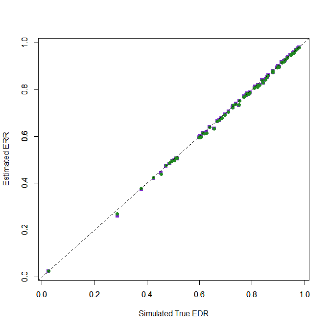
These results merely confirm that extensive simulation studies by Brunner and Schimmack (2020) showed. ERR estimates are f^&%%$ good. The scientific way to say this is to compute the root mean square error (RMSE) for the difference between true and expected ERR values. The RMSE for the OF method is .007. The value for the EM method is also .007.

The minimum directional error was -2.7 percentage points for OF and -2.3 percentage points for EM. The maximum was 0.4 for OF and 0.3 for EM. These differences have no practical significance in any estimates of the ERR.

It is not clear how they stumbled on a limited number of scenarios that all showed poor performance. Here I showed that z-curve predicts true values of the ERR n 66 simulations that cover the full range of average power. These simulations were not chosen to produce good performance because they represent a complete design. Moreover, you can use the R-code to test other scenarios, as we have done in many other simulations without finding notable biases in ERR estimates.

Expected Discovery Rate

Estimating the discovery rate solely on the basis of the distribution of significant z-values is harder. As a result, the estimates are not as good as the ERR estimates, but how good or bad are they?

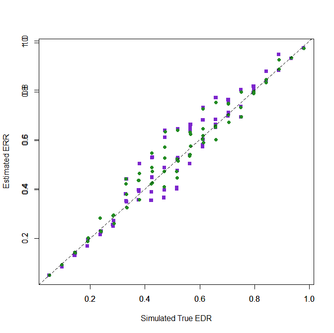
Visual inspection of the plot shows biases for medium power, whereas high and low EDR estimates are better. The RMSE values show slightly better performance for the “EM” method, RMSE = .051 than the OF method, RMSE = .063. It is therefore recommended to use the “EM” method for final results.

The biggest underestimation / downward bias was -11 percentage points for OF and -7 percentage points for EM. The biggest overestimation / upward bias was 17% for OF and 16% for EM.

The next figure shows a follow-up simulation for the scenario with the largest overestimation (Simulation #41). To reduce sampling error further, I used k = 200,000 studies and the fast OF method (takes about 5 seconds).

The bias is much smaller showing that z-curve estimates of the EDR also have high large-sample accuracy and that the larger bias in the previous simulation was still influenced by sampling error. Of course, real datasets are smaller and will produce biased estimates, but that will be reflected in wide confidence intervals; a topic for another chapter.

The biggest upward bias was observed in a condition when most values were from the z2 component.

Conclusion

Motivated biases are one of the best documented examples in psychology. Simulation studies help researchers to test their intuitions against reality. I have learned a lot from simulations. However, in public simulations are often used to sell a specific method, or apparently to discredit a specific method by picking scenarios that work well or where a method performs poorly. It is therefore best to see the performance of a method with your own eyes. This tutorial makes it easy to run simulation studies and with a bit of R-coding or help from an AI to modify the simulation to try out other scenarios.

These results are limited to simulations with normal distributions and do not address uncertainty of estimates in smaller samples. Thus, good performance in these simulations is necessary, but not sufficient to trust z-curve results “in the wild.” Necessary means that bad performance in these simulations would have been the end of z-curve. Z-curve only exists because it does well in these simulations. Insufficient means that we need other simulations that are similar to real data to see how it performs in these settings.

At the same time, these results are sufficient to point out that some academics (teachers at universities, but not scientists who follow a code of ethics) make false claims about the performance of z-curve that are falsified by the evidence in published articles and the results in this tutorial. ..

“To date, we have only examined a limited set of scenarios. Yet, we have found relatively few instances in which estimates from the typical use of the 𝑍-curve approach (i.e., analyzing only 𝑝-values < .05) have performed well.”

So, this tutorial also taught you the importance of evaluating conflicting claims based on scientific evidence. Never trust a scientist. Trust the science. When you ask an AI, always ask for the supporting evidence and ask it to challenge itself. Often AI is more trustworthy because it does not love or hate z-curve. It doesn’t give a shit about z-curve and that makes it a better judge of z-curve’s performance.