In an ideal world, humans would curb self-interest for the greater good. In reality, psychology has shown that human information processing is riddled with self-serving biases. A great achievement of human cultural evolution is the development of tools that can reduce these biases such as logical thinking and objective empirical observations. Since the invention of computers, it has also become easier to use simulations to put intuition to a test. However, motivated self-interest can bias simulations to produce desirable outcomes. For example, Uri Simonsohn made unreasonable assumptions to claim that p-curve performs well even with heterogeneity in power (Schimmack, 2018). It does not (Brunner,

An anonymous reviewer, henceforth known as Reviewer A (which may stand for anonymous or another word starting with A), recently accused us that we also used biased simulations to make the false claim that z-curve provides useful estimates of power with good coverage of confidence intervals (Brunner & Schimmack, 2020; Bartos & Schimmack, 2022; Schimmack & Bartos, 2023). The same reviewer previously made numerous false claims about z-curve and estimation of true power that we addressed elsewhere (Brunner, 2024). In our response to Reviewer A’s earlier comments, we also challenged them to provide a simulation that shows when z-curve breaks down.

Reviewer A was able to do so. The question is how they did it and whether Reviewer A’s results challenge our simulation results. Here is Reviewer A’s simulation.

To show that z-curve breaks down without hodgepodge heterogeneity, let us consider a situation of unconditional power of value .25   We have a one-sample Cohen’s d population value ranging from 0.2 to 2.2 (by increments of .05 to end up with 40 values), that is accompanied by sample size ranging from 167 to 2 that is calculated to be associated with a power of .25.

I generated data from each combination of Cohen’s d and sample size and fit a paired-samples t-test to obtain 40 p-values. These p-values are associated with a (“unconditional”) power value of .25. The expected discovery rate should be .25 (which is the power associated with the design of these observed results). The output I obtain from the zcurve package for the 40 estimated p-values is 0.05 – very far from the true value of .25.

To be clear, an estimate of 5% power (no evidence against the null-hypothesis) when the true power is 25% is horrible. So, we need to examine the conditions that lead to this horrible outcome. Here is Reviewer A’s code.

R code
d <- seq(.2,2.2,by = 0.05) # range of population Cohen’s d value
ssize<- matrix (0, ncol=40,nrow=1) #placeholder for sample size
pow = .25 #change this to change level of true power
for (i in 1:40){ #obtain sample size associated with Cohen’s d value for chosen level of power.
  ssize [i] <- pwr.t.test(n = NULL, d = d[i], sig = .05, power = pow,
                          type=”one.sample”, alternative=”two.sided”)$n
}
ssize_ <- round(ssize,digits=0) #round up the values
pp <- matrix(0,ncol=40,nrow=1)  #placeholder for estimated p-values
#let’s generate data and collect p-values
for (i in 1: 40){
  dat <- rnorm(n=ssize_[i], mean=d[i], sd=1)
  pp[i] <- t.test(dat, paired=FALSE, alternative=”two.sided”)$p.value
}
*let’s use zcurve to see whether EDR reproduces the specified power value
zcurve(p=as.vector(pp))
==

Let’s first address an annoying side issue in this simulation. The simulation is based on 40 simulated studies or test results. With power of 25% only about 10 of those are expected to be significant and useful for a z-curve analysis to estimate power. We have warned that z-curve estimates with small k (k = 10; 10 p-values below .05) are too variable to be meaningful. They also have wide confidence intervals that Reviewer A does not bother to report. However, this is a side-issue. We can simply increase the number of tests from 40 to 100,000 and see the large-sample bias in z-curve estimates. This confirms that z-curve severely underestimates power in this simulation. So, let’s take a closer look at the scenario that is being simulated.

The simulation starts with effect sizes ranging from small (d = .2) to effect sizes that are very large and rarely observed in real studies (d = 2.2). It is well known that power increases with larger effect sizes. Thus, to maintain low power of 25%, we have to reduce sample sizes. The sample sizes implied by this simulation are as follows.

N freq. perc.
2 11 26.8%
3 13 31.7%
4 4 9.8%
5 3 7.3%
6 1 2.4%
7 2 4.9%
9 1 2.4%
10 1 2.4%
12 1 2.4%
15 1 2.4%
20 1 2.4 %
28 1 2.4%
43 1 2.4%

These results show that only 10% of studies had sample sizes of 15 or more participants and over half of the simulated studies had 2 or 3 participants. As the simulation focused on a one-sample t-test, a study with N = 2 has 1 degree of freedom. This important information was hidden from the editor who is supposed to make decisions based on peer-reviewers’ comments.

Reviewer A could have just simulated studies with sample sizes of 2 or 3 participants to show that z-curve does not work well with these sample sizes, but maybe the editor would have noticed that this is not a reasonable assumption because most studies have more than 3 participants. In fact most studies have more than 20 participants. So, the only plausible reason to simulate effect sizes, when sample size is the driving factor is to hid explicit information about sample sizes from readers who do not understand t-distributions very well.

That being said, it is interesting to examine whether small sample sizes that are actually found in research articles still bias z-curve estimates. For example, John Bargh’s infamous elderly priming study that could not be replicated had only n = 15 participants in the control and experimental group for a total of N = 30 and 28 degrees of freedom. Would z-curve estimates underestimate power with these small sample sizes? Before I can present the results, it is important to point out that z-curve provides to estimates of power. One is the estimated power (including power of 5% for studies where the null-hypothesis is true) of all studies that were conducted and produced significant and non-significant results. This is called the expected discover rate. The second estimate is the power of the subset of studies that produced a significant result (including false positive results with power of 5%, if alpha is set to .05). This is called the expected replication rate because it predicts how many significant results would be obtained if only the studies with significant results were replicated exactly, including the original sample sizes. When power is fixed, the true EDR and ERR are the same, but estimates and biases can differ because estimating the EDR is more difficult.

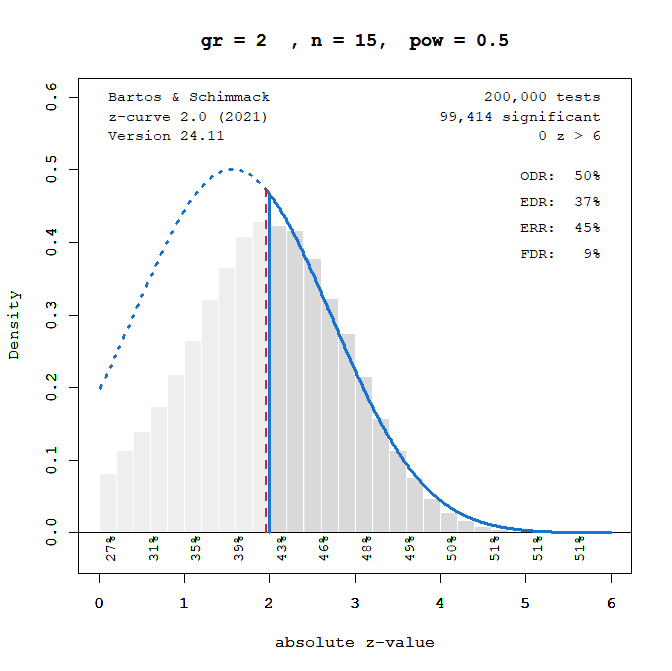
We can use Reviewer A’s code to determine the effect size that is needed to get significance in a simple between-group study with n = 15 per group (Bargh also had a covariate which increases power, but that is not relevant here). I simulated power of 50%.

#Note. pwr uses n of a single group. with n=15 and type=two.sample, the total N=30 and df =28
d <- pwr.t.test(n = 15, d = NULL, sig = .05, power = .50,
                          type=”two.sample”, alternative=”two.sided”)$d

With N = 30 total sample size we need a large effect size of d = .74 to have 50% power.

Figure 1 shows the t-distribution from which test statistics of individual studies are sampled (green). It also shows the standard normal distribution that is implied by 50% power (black). Visual inspection shows that the two distributions are similar but not identical.

The approximation of the asymmetrical non-central t-distribution with the standard normal distribution introduces some bias in z-curve estimates. For this example, the true power of 50% is underestimated by 4 percentage point. More problematic is that the EDR is underestimated by 13 percentage points. This finding suggests that estimates of the EDR and the FDR, which is simply a transformation of the EDR, are biased in sets of studies with small sample sizes (N < 30), even if we disregard silly sample sizes of N = 2.

Is there a solution to this problem? Indeed there is one and maybe we should have thought about it before, but as they say “better late than never.” There is an alternative approach to ‘convert’ t-values into z-scores. (or F-values with df = 1, t = F^2, i.e., t is the square root of the F-value or F-values are simply squared t-values). The alternative is to simply use the t-value as an estimate of z-scores.

ChatGPT: How to convert t-values into z-scores?

Find the cumulative probability of the t-value: Use a t-distribution table or statistical software to find the p-value associated with the t-value given your specific degrees of freedom. This p-value represents the area under the curve to the left of your t-value (for a one-sided test) or half the area in a two-tailed test. Once you have the p-value, use the inverse of the standard normal distribution (Φ⁻¹) to find the corresponding z-score.

Alternative Formula (if df > 30): For degrees of freedom over 30, the t-distribution closely resembles the normal distribution, so you can directly approximate the z-score by using the t-value.

It is clear that this approach will lead to overestimation of power (EDR, ERR) because uncorrected t-values with small degrees of freedom are always larger than the corresponding z-scores. The question is how big this bias is when we use this approach to conduct z-curve analyses. Here are the results for the same data, but the input are the uncorrected t-values.

The results for the ERR are as expected: the true power is overestimated. Interestingly, the bias is as strong as for the transformation approach, but in the opposite direction. This suggests a possible way to quantify the amount of bias, by using both approaches and use half of the difference in estimates as an estimate of the amount of bias. The results for the EDR are a bit more surprising. There is no bias in the estimate. The reason is that bias is introduced by the wide tail of the t-distribution and this tail has a weaker effect on power for all tests. This is a very encouraging finding and suggests that it is preferable to use this approach to submit t-values to z-curve.

Large sample bias is often hard to detect when the set of studies is small. Moreover, confidence intervals of z-curve estimates are adjusted to allow for small systematic biases. It is therefore interesting to compare the coverage of confidence intervals for both approaches. To do so, I split the 200,000 t-values into 1,000 sets of 200 observations and ran z-curve with confidence intervals. I then checked the percentage of confidence intervals that included the true parameter.

For the ERR, 94.7% of confidence intervals included the true parameter. This is just 0.3 percentage points more than we would expect from a 95% confidence interval. For sample sizes greater than 30, this would imply good coverage. For the EDR, 97.7% of confidence intervals included the true power, indicating good coverage for the 95% confidence interval.

We will follow up on these preliminary results with more extensive simulations, but the results suggest that it is preferable to use t-values as estimates of z-values rather than using the transformation by means of p-values. We also suggest to limit z-curve analysis to studies with at least N = 30 participants for now.

Conclusions about Z-Curve

Z-curve was developed as a statistical tool that estimates the average power of a set of studies. It does so for two populations of studies. One population is all studies that were conducted independent of the result. The other population is the subset of studies that produced a statistically significant result. Alternative methods exist, but z-curve is the only method that can be used when studies differ in power (heterogeneity) without having to make assumptions about the distribution of true power (Brunner & Schimmack, 2020).

As all methods that rely on samples to make claims about populations, z-curve cannot reveal the true average power. It can only provide estimates of average true power in a population of studies. There are two sources of uncertainty in these estimates. One is ordinary sampling error. The other is systematic bias that can be introduced by approximating test-statistics from different designs with z-values. Z-curve provides confidence intervals that take both sources of error into account. Simulation studies suggest that 95% confidence intervals contain the true parameter at least 95% of the time in many realistic scenarios.

Reviewer A’s simulations showed that this is no longer the case when sample sizes are small. A simple solution to this problem is not to include studies with very small sample sizes in z-curve analyses. At present, I would suggest to exclude studies with N < 30 or to be mindful if studies with smaller sample sizes are part of the set of studies. I also recommend a new approach to include t-values and F-values with one degree of freedom. instead of converting them to p-values, t-values should be directly used as estimates of z-values.

Conclusions about Peer Review, Scientific Integrity, and Reviewer A

After presenting misleading claims about statistical power that we have carefully examined and shown to be misguided (Brunner, 2024), Reviewer A uses the results of their dishonest simulation study to claim that z-curve is unable to estimate the true power of a set of studies.

In sum, I do not think that the z-curve delivers estimates of the expected discovery rate (and its sister concept of expected replication rate) on a conceptual basis. The arguments for using estimates of “unconditional power” seem not to reasonably justify making a claim on the discovery rate of a set of publications (why not just count up the p-values if p-values signal discovery?). Even if my conceptual points are swept under the rug (again), perhaps the simulated illustration showing that z-curve does not provide an estimate near to the true value of the “expected discovery rate” would be convincing. Why does it break? Well, that goes back to the conceptual issues I have pointed out about consistency and efficiency of observed power, and the hodgepodge problem of combining lots of things together and hoping all the bad stuff averages out.  One might choose to argue that z-curve can run but cannot walk (that is, it performs well enough in a complex case but fails miserably in simple cases). I would not be convinced of such an argument that ignores first principles.

To be fair, Reviewer A states “I do not think,” which suggests that they are open to the idea that they may be wrong. However, it is unclear why reviewer A continues to ignore the evidence presented in peer-reviewed articles and the opinions of several reviewers who did not see the fundamental problems that they see.  When there is differences in opinions about factual statements, it is important to examine the underlying thought processes and evidence. Reviewer A failed to do so (“I do not think”). Rather, Reviewer A has set up a biased simulation that confirms their suspicion and accuses us of doing the very same thing they were doing. (If this sounds familiar, you know that it can be an effective strategy to deceive people).

Why does z-curve break in the simulations? As I have shown in this blog post, it breaks down in the simulations by Reviewer A when we use it with sample sizes of N = 2 or 3, it is still biased with sample sizes of N = 30, and it does well with large sample sizes. Reviewer A hides the missing moderator (a.k.a., hidden moderator), sample size, which they are well aware off because they knew hot to break z-curve with sample sizes of N < 10. However, they falsely generalize from this unrealistic scenario to all applications with larger sample sizes and ignore that many simulations with larger sample sizes have shown that z-curve performs well.

This deception is not different from the questionable research practices that original researchers sometimes use to present statistically significant results without any real effects (Bem, 2011). They know more than they are telling their audience to present misleading scientific evidence for false claims. Just like Reviewer A’s dishonest behavior, questionable practices in peer-reviews are not rare exceptions, but common occurrences that are based on human’s struggle to overcome their own biases. This would not be a problem, if there were an open exchange of arguments between authors and reviewers that works out the causes of disagreement. Here it is easy to show that the original simulation and Reviewer A’s simulations are both correct and that sample size is the moderator. Once this is clarified, the editor can decide whether simulations based on N = 2 or N = 100 are more relevant. However, often editors are quick to reject articles based on the expert opinions of reviewers, especially in flashy journals that pride themselves on high rejection rates. It is not surprising that the quality of articles in these journals is not better than in other journals because experts will use their power to favor articles that agree with their opinions and be hypercritical about articles that do not. It is well known that pre-publication peer-review is very subjective and reviewers often disagree even about ratings of the quality of a literature review.

How can we improve peer-review? The answer is simple. Make them open! Open science requires transparency of all steps of the production of a scientific article, which includes peer-review. Some innovative journals have implemented open peer-reviews. We are proud that two z-curve articles have been published in the leading journal Meta-Psychology (conflict of interest declaration: I am co-founder of this journal with Rickard Carlsson who has been main editor since its inception). Reviewer A’s opinions do not just clash with our own opinions. They are also inconsistent with reviewers of z-curve who put their name next to their reviews. In contrast, reviewers in legacy journals hide their identity from the authors and the public. Just like I challenged Reviewer A to present a simulation to break z-curve, I challenge them here to an open exchange about the ability of z-curve to estimate the true power of a set of studies. Open exchange of arguments in real time (like in a chess game) in front of an audience needs to be added to the open science practices. Let’s make a badge for that and I will be happy to earn a few of those.