Abstract
Loken and Gelman published the results of a study that aimed to simulate the influence of random measurement error on effect size estimates in studies with low power (small sample, small correlation). Figure 3 suggested that “of statistically significant effects observed after error, a majority could be greater than in the “ideal” setting when N is small” I show with a simple simulation study that this result is based on a mistake in their simulation study that conflates sampling error and random measurement error. Holding random measurement error constant across simulations reaffirms Hausman’s iron law of econometrics that random measurement error is likely to produce attenuated effect size estimates. The article concludes with the iron law of meta-science. Original authors of a novel discovery are the least likely people to find an error in their work.

Introduction

Loken and Gelman published a brief essay on “Measurement error and the replication crisis” in the magazine Science. As it turns out, the claims in the article are ambiguous because key terms like measurement error are not properly defined. However, the article does contain the results of simulation studies that are presented in a Figure. The key figure is Figure 3.

This figure is used to support the claim that “of statistically significant effects observed after error, a majority could be greater than in the “ideal” setting when N is small.”

Some points about this claim are important. It is not a claim about a single study. In a single study, measurement error, sampling error, and other factors CAN produce a stronger result with a less reliable measures, just like some people can win the lottery, even though it is a very unlikely event. The claim is clearly about the outcome in the long-run after many repeated trials. That is also implied by a figure that is based on simulations of many repeated trials of the same study. What does the figure imply? It implies that measurement error attenuates observed correlations (or regression coefficients with measurement error in the predictor variable, x) in large samples. The reason is simply that random measurement error adds variance to a variable that is unrelated to the outcome measure. As a result, the observed correlation is a mixture of the true relationship and a correlation of zero and the mixture depends on the amount of random measurement error in the predictor variable.

Selection for significance on the other hand has the opposite effect. To obtain significance, the observed correlation has to have a minimum value so that the observed correlation is approximately twice as large as the sampling error (t ~ 2 equals p < .05, two-tailed). In large samples, sampling error is small and correlations of r = .15 are significant in most cases (i.e., the study has high power). When 99% of all studies are significant, selecting for significance to get a success rate of 100% is irrelevant. However, in small samples with N = 50, a small correlation of r = .15 is not enough to get significance. Thus, all significant correlations are inflated. Measurement error attenuates correlations and makes it even harder to get significant results. With reliability = .8 and a correlation of r = .15, the expected correlation is only .15 * .8 = .12 and more inflation is needed to get significance.

Figure 3 in Loken and Gelman’s article suggests that selection for significance with unreliable measures produces even more inflated effect size estimates than selection for significance without measurement error. This is implied by the results of a simulation study that produced a majority (over 50%) of outcomes where the effect size estimate was higher (and more inflated) when random measurement error was added than in the ideal setting without random measurement error. Loken and Gelman’s claim “of statistically significant effects observed after error, a majority could be greater than in the “ideal” setting when N is small” is based on this result of their simulation studies. With N = 50, r = .15, and reliability of .8, a majority of the comparisons showed a stronger effect size estimate for the simulation with random error than for the simulation without random error.

I believe that this outcome is based on an error in their simulation studies. The simulation does not clearly distinguish between sampling error and random measurement error. I have tried to make this point repeatedly on Gelman’s blog post, but this discussion and my previous blog post (that Gelman probably did not read) failed to resolve this controversy. However, it helped me to understand the source of the disagreement more clearly. I maintain that Gelman does not make a clear distinction between sampling error (i.e., even with perfectly reliable measures, results will vary from sample to sample and this variability is larger in small samples, STATS101) and random measurement error (i.e., two measures of the same constructs are not perfectly correlated with each other, NOT A TOPIC OF STATISTCS, which typically assumes perfect measures). Based on this insight, I wrote a new r-script that clearly distinguishes between sampling error and random measurement error. I ran the script 10,000 times. Here are the key results.

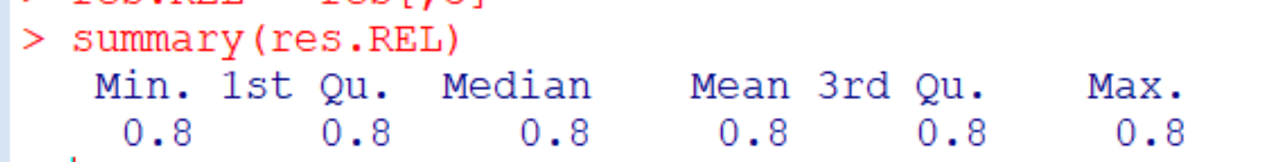
The simulation ensured that reliability in each run is exactly 80%.

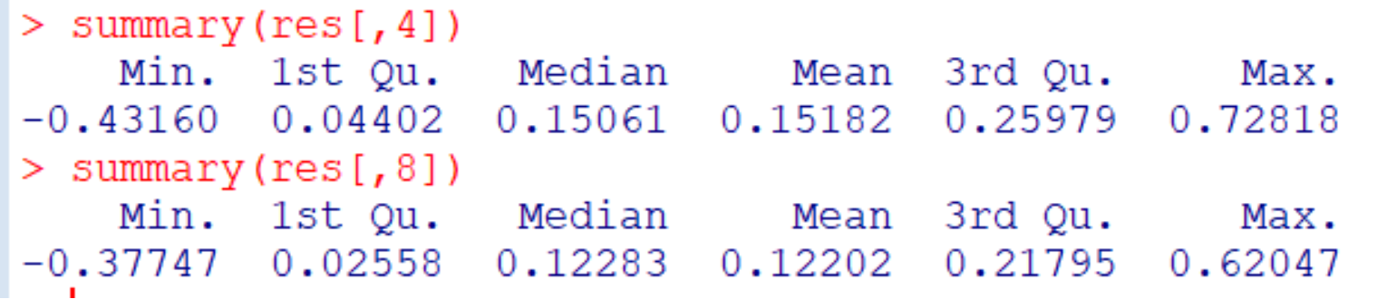
The expected effect sizes are r = .15 for the true relationship and r = .12 for the measure with 80% reliability. The average effect sizes across the 10,000 simulations match these expected values. We also see that sampling error produces huge variability in specific runs. However, even extreme deviations are attenuated by random measurement error. Thus, random measurement error makes values less extreme.

What about sign errors. We don’t really know the true correlation and two-tailed testing allows researchers to reject H0 with the wrong sign. To allow for this possibility, we can compute the absolute correlations.

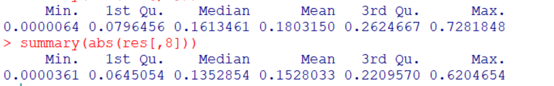
This does not matter. The results for the measure with random error are still lower and less extreme.

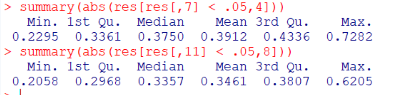
Now we can examine how conditioning on significance influences the results.

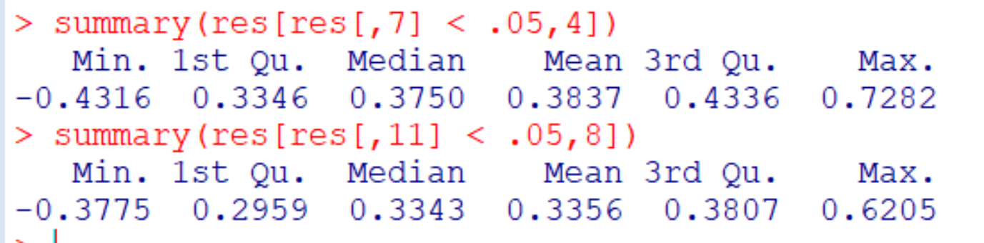
Once more the effect size estimates for the true correlation are stronger and more extreme than those for the measure with random measurement error. This is also true for absolute effect size estimates.

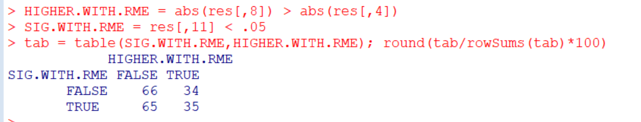
Loken and Gelman’s Figure 3 required the direct comparison of two outcomes in the same run after selection for significance. This creates a problem because sometimes one result will be significant and the other one will not be significant. As a result, the comparison is biased because it compares estimates after selection for significance with estimates without selection for significance. However, even with this bias in favor of the unreliable measure, random measurement error produced weaker effect size estimates in the majority of all cases.

Conclusion

In short, these results confirm Hausman’s iron law of econometrics that random measurement error typically attenuates effect size estimates. Typically, of course, does not mean always. However, Loken and Gelman claimed that they identified a situation in which the iron law of economics does not apply and can lead to false inferences. They claimed that (a) in small samples and (b) after selection for significance, random measurement error will produce stronger effect size estimates not once or twice but IN A MAJORITY of studies. This claim was implied by the results of their simulations displayed in Figure 3. Here is showed that their simulation fails to simulate the influence of random measurement error. Holding random measurement error constant at 80% produces the expected outcome that random measurement error is more likely to attenuate effect size estimates than to inflate it even in small samples and after selection for significance. Thus, researchers are justified to claim that they could have obtained stronger correlations with a more reliable measure or to use latent variable models to correct for unreliability. What they cannot do is to claim that the true population correlation is stronger than their observed correlation because this claim ignores the influence of selection for significance that inevitably inflates observed correlations in small samples with small effect sizes. It is also not correct to assume that two wrongs (selecting for significance with unreliable measures) make one right. Robust and replicable results require good data. Effect sizes of correlations should only be interpreted if measures have demonstrated good reliability (and validity, but that is another topic) and when sampling error is small enough to produce a meaningful range of plausible values.

New Simulation of Reliability

N = 50

REL = .80
n.sim = 10000

res = c()

for (i in 1:n.sim) {

SV = scale(rnorm(N))*sqrt(REL)
var(SV)

x1 = rnorm(N)
x1 = residuals(lm(x1 ~ SV))
x1 = scale(x1)
x1 = x1*sqrt(1-REL)
var(x1)

x2 = rnorm(N)
x2 = residuals(lm(x2 ~ x1 + SV))
x2 = scale(x2)
x2 = x2*sqrt(1-REL)
var(x2)

x1 = x1 + SV
x2 = x2 + SV

y = .15 * SV + rnorm(N)*sqrt(1-.15^2)

r = c(var(x1),var(x2),cor(x1,x2),
summary(lm(y ~ SV))$coef[2,],
summary(lm(y ~ x1))$coef[2,],
summary(lm(y ~ x2))$coef[2,]
);r

res = rbind(res,r)

} # End of sim

summary(res)