Abstract
Ulrich Orth, Angus Clark, Brent Donnellan, Richard W. Robins (DOI: 10.1037/pspp0000358) present 10 studies that show the cross-lagged panel model (CLPM) does not fit the data. This does not stop them from interpreting a statistical artifact of the CLPM as evidence for their vulnerability model of depression. Here I explain in great detail why the CLPM does not fit the data and why it creates an artifactual cross-lagged path from self-esteem to depression. It is sad that the authors, reviewers, and editors were blind to the simple truth that a bad-fitting model should be rejected and that it is unscientific to interpret parameters of models with bad fit. Ignorance of basic scientific principles in a high-profile article reveals poor training and understanding of the scientific method among psychologists. If psychology wants to gain respect and credibility, it needs to take scientific principles more seriously.
Introduction
Psychology is in a crisis. Researchers are trained within narrow paradigms, methods, and theories that populate small islands of researchers. The aim is to grow the island and to become a leading and popular island. This competition between islands is rewarded by an incentive structure that imposes the reward structure of capitalism on science. The winner gets to dominate the top journals that are mistaken as outlets of quality. However, just like Coke is not superior to Pepsi (sorry Coke fans), the winner is not better than the losers. They are just market leaders for some time. No progress is being made because the dominant theories and practices are never challenged and replaced with superior ones. Even the past decade that has focused on replication failures has changed little in the way research is conducted and rewarded. Quantity of production is rewarded, even if the products fail to meet basic quality standards as long as naive consumers of researchers are happy.
This post is about the lack of training in the analysis of longitudinal data with a panel structure. A panel study essentially repeats the measurement of one or several attributes several times. Nine years of undergradute and graduate training leave most psychologists without any training how to analyze these data. This explains why the cross-lagged panel model (CLPM) was criticized four decades ago (Rogosa, 1980), but researchers continue to use it with the naive assumption that it is a plausible model to analyze panel data. Critical articles are simply ignored. This is the preferred way of dealing with criticism by psychologists. Here, I provide a detailed critique of CLPM using Orth et al.’s data (https://osf.io/5rjsm/) and simulations.
Step 1: Examine your data
Psychologists are not trained to examine correlation matrices for patterns. They are trained to submit their data to pre-specified (cookie-cutter) models and hope that the data fit the model. Even if the model does not fit, results are interpreted because researchers are not trained in modifying cookie cutter models to explore reasons for bad fit. To understand why a model does not fit the data, it is useful to inspect the actual pattern of correlations.
To illustrate the benefits of visual inspection of the actual data, I am using the data from the Berkeley Longitudinal Study (BLS), which is the first dataset listed in Orth et al.’s (2020) table that lists 10 datasets.
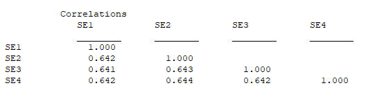
To ease interpretation, I break up the correlation table into three components, namely (a) correlations among self-esteem measures (se1-se4 with se1-se4), correlations among depression measures (de1-de4 with de1-de4), and correlations of self-esteem measures with depression measures (se1-se4 with de1-de4);

Table 1 shows the correlation matrix for the four repeated measurements of self-esteem. The most important information in this table is how much the magnitude of the correlations decreases along the diagonals that represent different time lags. For example, the lag-1 correlations are .76, .79, and .74, which approximately average to a value of .76. The lag-2 correlations are .65 and .69, which averages to .67. The lag-3 correlation is .60.
The first observation is that correlations are getting weaker as the time-lag gets longer. This is what we would expect from a model that assumes self-esteem actually changes over time, rather than just fluctuating around a fixed set-point. The latter model implies that retest correlations remain the same over different time lags. So, we do have evidence that self-esteem changes over time, as predicted by the cross-lagged panel model.
The next question is how much retest correlations decrease with increasing time lags. The difference from lag-1 to lag-2 is .74 – .67 = .07. The difference from lag-2 to lag-3 is .67 – .60, which is also .07. This shows no leveling off of the decrease in these data. It is possible that the next wave would produce a lag-4 correlation of .53, which would be .07 lower than then lag-3 correlation. However, a difference of .07 is not very different from 0, which would imply that change asymptotes at .60. The data are simply insufficient to provide strong information about this.
The third observation is that the lag-2 correlation is much stronger than the square of the lag-1 correlations, .67 > .74^2 = .55. Similarly, the lag-3 correlation is stronger than the product of the lag-1 and lag-2 correlations, .60 > .74 * .67 = .50 This means that a simple autoregressive model with observed variables does not fit the data. However, this is exactly the model of Orth et al.’s CLPM.
It is easy to examine the fit of this part of the CLPM model, by fitting an autoregressive model to the self-esteem panel data.
Model:
se2-se4 PON se1-3 ! This command regresses each measure on the previous measure (n on n-1).
! There is one thing I learned from Orth et al., and it was the PON command of MPLUS
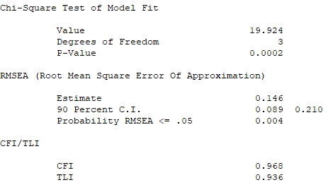
Table 2 shows the fit of the autoregressive model. While CFI meets the conventional threshold of .95 (higher is better), RMSEA shows terrible fit of the model (.06 or lower are considered acceptable). This is a problem for cookie-cutter researchers who think CLPM is a generic model that fits all data. Here we see that the model makes unrealistic assumptions and we already know what the problem is based on our inspection of the correlation table. The model predicts more change than the data actually show. We are therefore in a good position to reject the CLPM as a viable model for these data. This is actually a positive outcome. The biggest problem in correlational research are data that fit all kinds of models. Here we have data that actually disconfirm some models. Progress can be made, but only if we are willing to abandon the CLPM.
Now let’s take a look at the depression data, following the same steps as for the self-esteem data.

The average lag-1 correlation is .43. The average lag-2 correlaiton is .45, and the lag-3 correlation is .4. These results are problematic for an autoregressive model because the lag-2 correlation is not even lower than the lag-1 correlation.
Once more it is hard to tell, whether retest-correlations are approaching an asymptote. In this case, the lag-2 minus lag-1 difference is -.02 and the lag-3 minus lag-2 difference is .05.
Finally, it is clear that the autoregressive model with manifest variables overestimates change. The lag-2 correlation is stronger than the square of the lag-1 correlations, .45 > .43^2 = .18, and the lag-3 correlation is stronger than the lag-1 * lag-2 correlation, .40 > .43*.45 = .19.
Given these results, it is not surprising that the autoregressive model fits the data even less than for the self-esteem measures (Table 4).
Model:
de2-de4 PON de1-de3 ! regress each depression measure on the previous one.
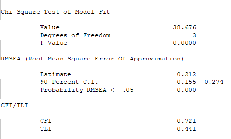
Even the CFI value is now in the toilet and the RMSEA value is totally unacceptable. Thus, the basic model of stability and change implemented in CLPM is inconsistent with the data. Nobody should proceed to build a more complex, bivariate model if the univariate models are inconsistent with the data. The only reason why psychologists do so all the time is that they do not think about CLPM as a model. They think CLPM is like a t-test that can be fitted to any panel data without thinking. No wonder psychology is not making any progress.
Step 2: Find a Model That Fits the Data
The second step may seem uncontroversial. If one model does not fit the data, there is probably another model that does fit the data and this model has a higher chance of being the model that reflects the causal processes that produced the data. However, psychologists have an uncanny ability to mess up even the simplest steps in data analysis. They have convinced themselves that it is wrong to fit models to data. The model has to come first so that the results can be presented as confirming a theory. However, what is the theoretical rational of the CLPM? It is not motivated by any theory of development, stability, or change. It is as atheoretical as any other model. It only has the advantage that it became popular on an island of psychology and now people use it without being questioned about it. Convention and conformity are not pillars of science.
There are many alternative models to CLPM that can be tried. One model is 60 years old and was introduced by Heise (1969). It is also an autoregressive model, but it also allows for occassion specific variance. That is, some factors may temporarily change individuals’ self-esteem or depression without any lasting effects on future measurements. This is a particularly appealing idea for a symptom checklist of depression that asks about depressive symptoms in the past four weeks. Maybe somebody’s cat died or it was a midterm period and depressive symptoms were present for a brief period, but these factors have no influence on depressive symptoms a year later.
I first fitted Heise’s model to the self-esteem data.
MODEL:
sse1 BY se1@1;
sse2 BY se2@1;
sse3 BY se3@1;
sse4 BY se4@1;
sse2-sse4 PON sse1-sse3 (stability);
se1-se4 (se_osv) ! occasion specific variance in self-esteem
Model fit for this model is perfect. Even the chi-square test is not significant (which in SEM is a good thing, because it means the model closely fits the data).

Model results show that there is significant occasion specific variance. After taking this variance into account the stability of the variance that is not occassion-specific, called state variance by Heise, is around r = .9 from one occasion to the next.

Fit for the depression data is also perfect.

There is even more occasion specific variance in depressive symptoms, but the non-occasion-specific variance is even more stable as the non-occasion-specific variance in self-esteem.

These results make perfect sense if we think about the way self-esteem and depression are measured. Self-esteem is measured with a trait measure of how individuals see themselves in general, ignoring ups and downs and temporary shifts in self-esteem. In contrast, depression is assessed with questions about a specific time period and respondents are supposed to focus on their current ups and downs. Their general disposition should be reflected in these judgments only to the extent that it influences their actual symptoms in the past weeks. These episodic measures are expected to have more occasion specific variance if they are valid. These results show that participants are responding to the different questions in different ways.
In conclusion, model fit and the results favor Heise’s model over the cookie-cutter CLPM.
Step 3: Putting the two autoregressive models together
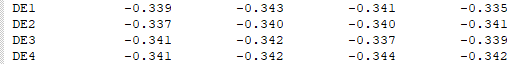
Let’s first examine the correlations of self-esteem measures with depression measures.
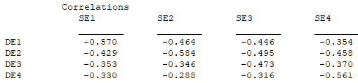
The first observation is that the same-occasion correlations are stronger (more negative) than the cross-occasion correlations. This suggests that occasion specific variance in self-esteem is correlated with occasion specific variance in depression.
The second observation is that the lagged self-esteem to depression correlations (e.g., se1 with de2) do not become weaker (less negative) with increasing time lag, lag-1 r = -.36, lag-2 r = -.32, lag-3 r = .33.
The third observation is that the lagged depression to self-esteem correlations (e.g., de1 with se2) do not decrease from lag-1 to lag-2, although they do become weaker from lag-2 to lag-3, lag-1 r = -.44, lag-2 r = -.45, lag-3 r = -.35.
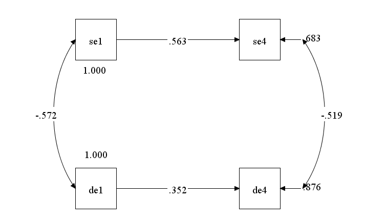
The fourth observation is that the lagged self-esteem to depression correlations (se1 with de2) are weaker than the lagged depression to self-esteem (de1 with se2) correlations . This pattern is expected because self-esteem is more stable than depressive symptoms. As illustrated in the Figure below, the path from de1-se4 is stronger than the path form se1 to de4 because the path from se1 to se4 is stronger than the path from de1 to de4.
Regression analysis or structural equation modeling is needed to examine whether there are any additional lagged effects of self-esteem on depressive symptoms. However, a strong cross-lagged path from se1 to de4 would produce a stronger correlation of se1 and de4, if stability were equal or if the effect is strong. So, a stronger lagged self-esteem to depression correlation than a lagged depression to self-esteem correlation would imply a cross-lagged effect from self-esteem to depression, but the reverse pattern is inconclusive because self-esteem is more stable.
Like Orth et al. (2020) I found that Heise’s model did not converge. However, unlike Orth et al. I did not conclude from this finding that the CLPM model is preferable. After all, it does not fit the data. Model convergence is sometimes simply a problem of default starting values that work for most models but not for all models. In this case, the high stability of self-esteem produced a problem with default starting values. Just setting this starting value to 1 solved the convergence problem and produced a well-fitting result.

The model results show no negative lagged prediction of depression from self-esteem. In fact, a small positive relationship emerged, but it was not statistically significant.

It is instructive to compare these results with the CLPM results. The CLPM model is nested in the Heise model. The only difference is that the occasion-specific variances of depression and self-esteem are fixed to zero. As these parameters were constrained across occasions, this model has two fewer parameters and the model df increase from 24 to 26. Model fit decreased in the more parsimonious model. However, the overall fit is not terrible, although RMSEA should be below .06 [Interestingly, the CFI value changed from a value over .95 to a value .94 when I estimated the model with MPLUS8.2, whereas Orth et al. used MPLUS8]. This shows the problem of relying on overall fit to endorse models. Overall fit is often good with longitudinal data because all models predict weaker correlations over longer time intervals. The direct model comparison shows that the Heise model is the better model.

In the CLPM model, self-esteem is a negative lagged predictor of depression. This is the key finding that Orth and colleagues have been using to support the vulnerability model of depression (low self-esteem leads to depression).

Why does the CLPM model produce negative lagged effects of self-esteem on depression. The reason is that the model underestimates the long-term stability of depression from time 1 to time 3 and time 4. To compensate for this it can use self-esteem that is more stable and then link self-esteem at time 2 with depression at time 3 (.745 * -.191) and self-esteem at time 3 with depression at time 4 (.742 * .739 * -.190). But even this is not sufficient to compensate for the misprediction of depression over time. Hence, the worse fit of the model. This can be seen by examining the model reproduced correlation matrix in the MPLUS Tech1 output.

Even with the additional cross-lagged path, the model predicts only a correlation of r = .157 from de1 to de4, while the observed correlation was r = .403. This discrepancy merely confirms what the univariate models showed. A model without occasion-specific variances underestimates long-term stability.
Interem Conclusion
Closer inspection of Orth et al.’s data shows that the CLPM does not fit the data. This is not surprising because it is well-known that the cross-lagged panel model often underestimates long-term stability. Even Orth has published univariate analyses of self-esteem that show a simple autoregressive model does not fit the data (Kuster & Orth, 2013). Here I showed that using the wrong model of stability creates statistical artifacts in the estimation of cross-lagged path coefficients. The only empirical support for the vulnerability model of depression is a statistical artifact.
Replication Study
I picked the My Work and I (MWI) dataset for a replication study. I picked it because it used the same measures and had a relatively large sample size (N = 663). However, the study is not an exact or direct replication of the previous one. One important difference is that measurements were repeated every two months rather than every year. The length of the time interval can influence the pattern of correlations.

There are two notable differences in the correlation table. First, the correlations increase with each measurement from .782 for se1 with se2 to .871 from se4 to se5. This suggests a response artifact, such as a stereotypic response styles that inflates consistency over time. This is more likely to happen for shorter intervals. Second, the difference between correlations with different lags are much smaller. They were .07 in the previous study. Here the differences are .02 to .03. This means there is hardly any autoregressive structure, suggesting that a trait model may fit the data better.
The pattern for depression is also different from the previous study. First, the correlations are stronger, which makes sense, because the retest interval is shorter. Somebody who suffers from depressive symptoms is more likely to still suffer two months later than a year later.

There is a clearer autoregressive structure for depression and no sign of stereotypic responding. The reason could be that depression was assessed with a symptom checklist that asks about the previous four weeks. As this question covers a new time period each time, participants may avoid stereotypic responding.

The depression-self-esteem correlations also become stronger (more negative) over time from r = -.538 to r = -.675. This means that a model with constrained coefficients may not fit the data.
The higher stability of depression explains why there is no longer a consistent pattern of stronger lagged depression to self-esteem correlations (de1 with se2) above the diagonal than self-esteem to depression correlations (se1 with de2) below the diagonal. Five correlations are stronger one way and five correlations are stronger the other way.
For self-esteem, the autoregressive model without occasion-specific variance had poor fit (RMSEA = .170, CFI = .920). Allowing for occasion-specific variance improved fit and fit was excellent (RMSEA = .002, CFI = .999). For depression, the autoregressive model without occasion-specific variance had poor fit (RMSEA = .113, CFI = .918). The model with occasion-specific variance fit better and had excellent fit (RMSEA = .029, CFI = .995). These results replicate the previous results and show that CLPM does not fit because it underestimates stability of self-esteem and depression.
The CLPM model also had bad fit in the original article (RMSEA = .105, CFI = .932). In comparison, the model with occasion specific variances had much better fit (RMSEA = .038, CFI = .991). Interestingly, this model did show a small, but statistically significant path from self-esteem to depression (effect size r = -.08). This raises the possibility that the vulnerability effect may exist for shorter time intervals of a few months, but not for longer time intervals of a year or more. However, Orth et al. do not consider this possibility. Rather, they try to justify the use of the CLPM to analyze panel data even though the model does not fit.
FITTING MODELS TO THEORIES RATHER THAN DATA
Orth et al. note “fit values were lowest for the CLPM” (p. 21) with a footnote that recognizes the problem of the CLPM, “As discussed in the Introduction, the CLPM underestimates the long-term stability of constructs, and this issue leads to misfit as the number of waves increases” (p. 63).
Orth et al. also note correctly that the cross-lagged effect of self-esteem on depression emerges more consistently with the CLPM model. By now it is clear why this is the case. It emerges consistently because it is a statistical artifact produced by the underestimation of stability in depression in the CLPM model. However, Orth et al.’s belief in the vulnerability effect is so strong that they are unable to come to a rational conclusion. Instead they propose that the CLPM model, despite its bad fit, shows something meaningful.
“We argue that precisely because the prospective effects tested in the CLPM are also based on between-person variance, it may answer questions that cannot be assessed with models that focus on within-person effects. For example, consider the possible effects of warm parenting on children’s self-esteem (Krauss, Orth, & Robins, 2019): A cross-lagged effect in the CLPM would indicate that children raised by warm parents would be more likely to develop high self-esteem than children raised by less warm parents. A cross-lagged effect in the RI-CLPM would indicate that children who experience more parental warmth than usual at a particular time point will show a subsequent increase in self-esteem at the next time point, whereas children who experience less parental warmth than usual at a particular time point will show a subsequent drop in self-esteem at the next time point”
Orth et al. then point out correctly that the CLPM is nested in other models and makes more restrictive assumptions about the absence of occasion specific variance or trait variance, but they convince themselves that this is not a problem.
As was evident also in the present analyses, the fit of the CLPM is typically not as good as the fit of the RI-CLPM (Hamaker et al., 2015; Masselink, Van Roekel, Hankin, et al., 2018). It is important to note that the CLPM is nested in the RI-CLPM (for further information about how the models examined in this research are nested, see Usami, Murayama, et al., 2019). That is, the CLPM is a special case of the RI-CLPM, where the variances of the two random intercept factors and the covariance between the random intercept factors are constrained to zero (thus, the CLPM has three additional degrees of freedom). Consequently, with increasing sample size, the RI-CLPM necessarily fits significantly better than the CLPM (MacCallum, Browne, & Cai, 2006). However, does this mean that the RI-CLPM should be preferred in model selection? Given that the two models differ in their conceptual meaning (see the discussion on between- and within-person effects above), we believe that the decision between the CLPM and RI-CLPM should not be based on model fit, but rather on theoretical considerations.
As shown here, the bad fit of CLPM is not an unfair punishment of a parsimonious model. The bad fit reveals that the model fails to model stability correctly. To disregard bad fit and to favor the more parsimonious model even if it doesn’t fit makes no sense. By the same logic, a model without cross-lagged paths would be more parsimonious than a model with cross-lagged paths and we could reject the vulnerability model simply because it is not parsimonious. For example, when I fitted the model with occasion specific variances and without cross-lagged paths, model fit was better than model fit of the CLPM (RMSEA = .041 vs. RMSEA = .109) and only slightly worse than model fit of the model with occasion specific variance and cross-lagged paths (RMSEA = .040).
It is incomprehensible to methodologists that anybody would try to argue in favor of a model that does not fit the data. If a model consistently produces bad fit, it is not a proper model of the data and has to be rejected. To prefer a model because it produces a consistent artifact that fits theoretical preferences is not science.
Replication II
Although the first replication mostly confirmed the results of the first study, one notable difference was the presence of statistically significant cross-lagged effects in the second study. There are a variety of explanations for this inconsistency. The lack of an effect in the first study could be a type-II error. The presence of an effect in the first replication study could be a type-I errror. Finally, the difference in time intervals could be a moderator.
I picked the Your Personality (YP) dataset because it was the only dataset that used the same measures as the previous two studies. The time interval was 6 months, which is in the middle of the other two intervals. This made it interesting to see whether results would be more consistent with the 2-month or the 1-year intervals.
For self-esteem, the autoregressive model with occasion specific variance had a good fit to the data (RMSEA = .016, CFI = .999). Constraining the occasion specific variance to zero reduced model fit considerably (RMSEA = .160, CFI = .912). Results for depression were unexpected. The model with occasion specific variance showed non-significant and slightly negative residuals for the state variances. This finding implies that there are no detectable changes in depression over time and that depression scores only have a stable trait and occasion specific variance. Thus, I fixed the autoregressive parameters to 1 and the residual state variances to zero. This model is equivalent to a model that specifies a trait factor. Even this model had barely acceptable fit (RMSEA = .062, CFI = .962). Fit could be increased by relaxing the constraints on the occasion specific variance (RMSEA = .060, CFI = .978). However, a simple trait model fit the data even better (RMSEA = .000, CFI = 1.000). The lack of an autoregressive structure makes it implausible that there are cross-lagged effects on depression. If there is no new state variance, self-esteem cannot be a predictor of new state variance.
The presence of a trait factor for depression suggests that there could also be a trait factor for self-esteem and that some of the correlations between self-esteem and depression are due to correlated traits. Therefore I added a trait factor to the measurement model of self-esteem. This model had good fit (RMSEA = .043, .993) and fit was superior to the CLPM (RMSEA = .123, CFI = .883). The model showed no significant cross-lagged effect from self-esteem to depression and the parameter estimate was positive rather than negative, .07. This finding is not surprising given the lack of decreasing correlations over time for depression.
Replication III
The last openly shared datasets are from the California Families Project (CFP). I first examined the children’s data (CFP-C) because Orth et al. (2020) reported a significant vulnerability effect with the RI-CLPM.
For self-esteem, the autoregressive model without occasion-specific variance had bad fit (RMSEA = .108, CFI = .908). Even the model with occasion-specific variance had poor fit (RMSEA = .091, CFI = .945). In contrast, a model with a trait factor and without occasion specific variance had good fit (RMSEA = .023, CFI = .997). This finding suggests that it is necessary to include a stable trait factor to model stability of self-esteem correctly in this dataset.
For depression, the autoregressive model without occasion-specific variance had bad fit (RMSEA = .104, CFI = .878). Even the model with occasion-specific variance had poor fit (RMSEA = .103, CFI = .897). Adding a trait factor produced a model with acceptable fit (RMSEA = .051, CFI = .983).
The trait-state model fit the data well (RMSEA = .989, CFI = .032) and much better than the CLPM (RMSEA = .079, CFI = .914). The autoregressive effect of self-esteem on depression was not significant, and only have the size of the effect size in the RI-CLPM ( -.05 vs. -.09). The difference is due to the constraint on the trait factor. Relaxing these constraints improves model fit and the vulnerability effect becomes non-significant.
Replication IV
The last dataset is based on the mothers’ self-reports in the California Families Project (CFP-M).
For self-esteem, the autoregressive model without occasion-specific variance had bad fit (RMSEA = .139, CFI = .885). The model with occasion specific variance improved fit (RMSEA = .049, CFI = .988). However, the trait-state model had even better fit (RMSEA = .046, CFI = .993).
For depression, the autoregressive model without occasion-specific variance had bad fit (RMSEA = .127, CFI = .880). The model with occasion-specific variance had excellent fit (RMSEA = .000, CFI = 1.000). The trait-state model also had excellent fit (RMSEA = .000, CFI = 1.000).
The CLPM had bad fit to the data (RMSEA = .092, CFI = .913). The Heise model improved fit (RMSEA = .038, CFI = .987). The trait-state model had even better fit (RMSEA = .031, CFI = .992). The cross-lagged effect of self-esteem on depression was negative, but small and not significant, -.05 (95%CI = -.13 to .02).
Simulation Study 1
The first simulation demonstrates that a cross-lagged effect emerges when the CLPM is fitted to data with a trait factor and one of the constructs has more trait variance which produces more stability over time.
I simulated 64% trait variance and 36% occasion-specific variance for self-esteem.
I simulated 36% trait variance and 64% occasion-specific variance for depression.

The correlation between the two trait factors was r = -.7. This produced manifest correlations of r = -.71*sqrt(.36)*sqrt(.64) = -.7 * .6 * .8 = -.34.
For self-esteem the autoregressive model without occasion specific variance had bad fit (). For depression, the autoregressive model without occasion specific variance had bad fit. The CLPM model also had bad fit (RMSEA = .141, CFI = .820). Although the simulation did not include cross-lagged paths, the CLPM showed a significant cross-lagged effect from self-esteem to depression (-.25) and a weaker cross-lagged effect from depression to self-esteem (-.14).
Needless to say, the trait-state model had perfect fit to the data and showed cross-lagged path coefficients of zero.
This simulation shows that CLPM produces artificial cross-lagged effects because it underestimates long-term stability. This problem is well-known, but Orth et al. (2020) deliberately ignore it when they interpret cross-lagged parameters in CLPM with bad fit.
Simulation Study 2
The second simulation shows that a model with a significant cross-lagged path can fit the data, if this path is actually present in the data. The cross-lagged effect was specified as a moderate effect with b = .3. Inspection of the correlation matrix shows the expected pattern that cross-lagged correlations from se to de (se1 with de2) are stronger than cross-lagged correlations from de to se (se2 with de1). The differences are strongest for lag-1.

The model with the cross-lagged paths had perfect fit (RMSEA = .000, CFI = 1.000). The model without cross-lagged paths had worse fit and RMSEA was above .06 (RMSEA = .073, CFI = .968).
Conclusion
The publication of Orth et al.’s (2020 article in JPSP is an embarrassment for the PPID section of JPSP. The authors did not make an innocent mistake. Their own analyses showed across 10 datasets that CLPM does not fit their data. One would expect that a team of researchers would be able to draw the correct conclusion from this finding. However, the power of motivated reasoning is strong. Rather than admitting that the vulnerability model of depression is based on a statistical artifact, the authors try to rationalize why the model with bad fit should not be rejected.
The authors write “the CLPM findings suggest that individual differences in self-esteem predict changes in individual differences in depression, consistent with the vulnerability model” (p. 39).
This conclusions is blatantly false. A finding in a model with bad fit should never be interpreted. After all, the purpose of fitting models to data and to examine model fit is to falsify models that are inconsistent with the data. However, psychologists have been brainwashed into thinking that the purpose of data analysis is only to confirm theoretical predictions and to ignore evidence that is inconsistent with theoretical models. It is therefore not a surprise that psychology has a theory crisis. Theories are nothing more than hunches that guided first explorations and are never challenged. Every discovery in psychology is considered to be true. This does not stop psychologists from developing and supporting contradictory models, which results in an every growing number of theories and confusion. It is like evolution without a selection mechanism. No wonder psychology is making little progress.
Numerous critics of psychology have pointed out that nil-hypothesis testing can be blamed for the lack of development because null-results are ambiguous. However, this excuse cannot be used here. Structural equation modeling is different from null-hypothesis testing because significant results like a high Chi-square value and derived fit indices provide clear and unambiguous evidence that a model does not fit the data. To ignore this evidence and to interpret parameters in these models is unscientific. The fact that authors, reviewers, and editors were willing to publish these unscientific claims in the top journal of personality psychology shows how poorly methods and statistics are understood by applied researchers. To gain respect and credibility, personality psychologists need to respect the scientific method.
Dear Dr. Schimmack,
thank you very much for this comprehensive demonstration and step-by-step data analysis approach. I find your text a very valuable response to the Orth et al. (2020) paper.
Nonetheless, while reading your text, I got somewhat confused by the different models you used. You commented under “Step 3” that the Heise model was also presented by Orth et al.. However, I was unable to identify the model in the Orth et al. paper, probably because the model was named differently. Could you please explain which model in Orth et al.s analysis you are referring to.
What is more, I wonder if the trait-models you refer to later in the text is consistent with the RI-CLPM (or better a univariate analysis with random intercept and state-like residuals), or, if not, what the differences are. In general, I wonder what your results tell us with regard to the CLPM vs. RI-CLPM discussion that Orth et al. open up. Would your findings support the usage of RI-CLPM?
Thank you very much for your response.
Kind regards
Maria
Thank you for your question. The blog post probably needs a revision to be clearer. Essentially, there is a general model with three factors that have different names: (a) trait, stable factors, random intercept, (b) autoregressive, state, changing factors, and (c) error, state, occasion specific
The standard cross-lagged panel model (CLPM) only has factor (b). The Heise model has b and c. The trait-state or RI-CLMP has a and b. The full trait-state-error model has all three but it can be difficult to identify all three components.
CLMP does not fit the data. RI-CLMP or the Heise model fit better and alter the cross-lagged path coefficients.
Thank you for your response!
Lynn Cooper doesn’t care that Orth et al. has published several JPSP articles that interpret a statistical artifact as a substantial discovery. More concerning, even reviewers who understand the statistical issues seem to miss the simple point of my commentary: the authors do a model comparison, find that the trait-model fits better, and then prefer the classic CLRM model because it shows the artifact they have been interpreting for over a decade.
Dear Dr. Schimmack,
Thank you for allowing the Journal of Personality and Social Psychology: Personality Processes and Individual Differences (JPSP:PPID) to consider your commentary for publication. I was fortunate to receive thoughtful and detailed reviews from two individuals with substantial methodological expertise. Indeed, Reviewer 1 is well known for his/her work on longitudinal data analysis. I consider both reviewers to be even handed, fair minded, and balanced in their perspectives. Neither has an axe to grind here. For all of these reasons, I respect their individual and collective judgement and am grateful for their guidance.
Based on the input provided by the two reviewers, along with my own independent read of the Orth et al. published paper, the initial reviews of that paper, and of course your commentary, I am sorry to say that I have decided to reject your submission for publication in JPSP.
I will not belabor the reasons for this decision as both reviewers lay out the key issues in unambiguous and remarkably consistent terms. However, I will briefly summarize the primary concerns that swayed me.
First, as both reviewers point out, too little information was provided about how the simulations were conducted to enable confident evaluation. Moreover, although you provided the code upon request, both reviewers found the code lacking for reasons they spell out in their respective reviews. Second, as both reviewers highlight, simulating a single data set with a single set of parameters falls well short of a convincing simulation. To quote Reviewer 2, who identified himself as Aiden Wright, “Simulating a single data set with a single set of conditions is hardly demonstration of much of anything. It may be that the single set of conditions tested is indicative of a more general problem, or it may be that the specific set of conditions is a narrow case under which the issues the reviewer is trying to raise holds. If they [you] are interested in raising a general concern about how the RI-CLPM and CLPM manage certain data generating processes, a thorough simulation is
needed.” Third, as Reviewer 1 explains, although model fit is an important criterion, other criteria also merit consideration. Moreover, fit of multilevel models is more complex and nuanced than your commentary suggests. While neither of these concerns necessarily invalidates the general issue you raise, they suggest that your treatment of this issue is at best overly simplistic – which is highly problematic given the centrality of this issue to your critique. Finally, both reviewers commented on the unprofessional tone of your commentary, and found your characterization of the Orth et al. paper unbalanced and dismissive.
In short, both reviewers and I agree that your commentary falls short of the type and scope of contribution required for publication in JPSP, even as a commentary. On that point, it is worth noting that JPSP only rarely publishes comments, and that Editors are under no obligation to publish them. Moreover, comments are reviewed by more or less the same standards used for regular articles, one that emphasizes the scientific importance of the information uniquely contributed by the comment. This is a very high bar to clear, especially if no – or as in the present case, only very limited – new data are presented.
My decision to reject your commentary does not, however, mean that your point is without merit. Indeed, it is possible that a longer methodological paper grounded in a more scholarly and thorough review of the literature that presents a more comprehensive set of simulation studies delineating conditions under which CLPM and RI-CLPM do or do not adequately model the underlying data generating processes could constitute an important contribution to the literature. Whether JPSP would be the ideal outlet for such a paper is, however, debatable.
I am sorry that I cannot be more positive on this particular submission, but I thank you again for allowing me to evaluate your submission, and hope that you will continue to consider JPSP as an outlet for your future work.
Sincerely,
M. Lynne Cooper, PhD
Editor
Journal of Personality and Social Psychology: Personality Processes and Individual Differences
Reviewers’ comments:
Reviewer #1: Review of PSP-P-2020-2065, ” You shall not interpret parameter estimates if your model does not fit the data.”
Background
The analysis of the cross-lagged panel design has a long history with origins in econometrics and sociology (see e.g., Hsaio, 1986; Kessler & Greenberg, 1981 for early texts devoted to panel designs). Kenny (1975, Psych. Bull.) popularized the approach in psychology, followed by a strong critique by Ragosa (1980, Psych. Bull.). The past decade has seen great advances in the approach (Hsaio, 2014 in econometrics; wonderful work by scholars in like Hamaker, Voelkle, and Zyphur in psychology (many of these are cited by Orth et al) have greatly advanced our understanding of these models, although there is much work yet to be done.
Among the key issues that have arisen are the following:
(1) Differentiating between person effects from within person effects. Following Molenaar’s (2004, Measurement) manifesto, there has been increasing emphasis on differentiating between within person and between person relationships. The within person and between person relationships can be different, even opposite in sign (see Boker & Martin, 2018 for a typing example; Voelkle et al., 2018 for a clinical example, both Multivariate Behavioral Research). Many of our standard models confound the two types of relationships. Hamaker and Muthen (2020, Psychological Methods) and Hamaker et al. (2019, Multivariate Behavioral Research) discuss these issues.
(2) A resurgence of interest in estimating potential causal effects. Several modern approaches to causal inference (e.g., Hernan & Robins, 2020; Pearl, text, 2009) have emphasized that we are often interested in making causal statements. The necessary conditions to identify a statistical model and a causal model may be different (see Ahern, 2018; Hernan, 2018, American Journal of Public Health), leading to different assumptions necessary to estimate the statistical and the causal models (see Gische et al., online first, Structural Equation Modeling; Hamaker et al., 2015; Psychological Methods for panel designs). This interest often means that additional restrictions (e.g., stationarity) need to be placed on the model for proper causal inference. In addition, researchers in the within person tradition see causal effects operating primarily at the within person level. In this view the between person parameters conceptually may alter the within person relationships, but
appropriate models are only beginning to be developed. (Causal inference becomes particularly challenging when a variable is constant over time).
(3) A recognition that our traditional models like ANOVA, regression, structural equation modeling have typically assumed that the same relationships apply to everyone in the population (i.e., constant effects). We are increasingly trying to include parameters that permit individual differences in effects. Economists tend to prefer indicator (~dummy) variables for persons; psychologists tend to prefer random effects which require the assumption of a normal distribution of individual differences. Hamaker et al. (2015) add random intercepts to the basic cross lagged panel model to represent stable individual differences. Attempts are now being made to add random cross-lagged effects and random autoregressive effects. These additions make the statistical model extremely difficult to estimate (e.g., see Hamaker et al., 2015) and may ultimately require a Bayesian approach to make progress.
Review of Orth et al.
I have no association with Orth et al. In my opinion, Hamaker and Voelkle have done the best job of surfacing the issues of panel designs in the methodological literature. Orth et al. did a nice review of much of the literature to that date and discussed many of the important issues. They illustrated the methods using many of the current approaches on several different data sets collecting data on self-esteem and depression. Their paper is one of the best illustrations of the approaches using empirical data that I have seen. That is not to say that I agree with all of their conclusions by any means, but they do a fairly evenhanded job of presenting the concerns on both sides of the issue. For example, in my view, certain restrictions to achieve stationarity are necessary for proper causal inference, whereas they emphasize model convergence. They emphasize the precision of the standard errors, a criterion on which random effects models are inherently inferior even if
they represent the more realistic model. I suspect, but have not done the algebra to verify this, that the simple cross lagged panel model does not estimate a pure between subjects effect as they claim.
Review of Commentary
There is no evidence that the author(s) of the commentary have done a thorough scholarly review of the current literature on panel models. The central comparison of Orth et al. is between the single level CLPM model and the RI-CLPM model which changes the model to a multilevel structure in which random intercepts are estimated. I only glanced at the code (which was not annotated and therefore far less informative than it could be; I only rarely use Mplus code) but it did NOT seem to be estimating a two level multilevel model. The brief description in the text (p. 3) did not make the model clear; from the description I would infer (perhaps incorrectly) that the authors preferred something closer to Rolf Steyer’s trait state model (Cole et al., 2005; Hamaker et al., 2015, both Psychological Methods include discussions of these classes of models). It is not clear that the CLPM and the RI-CLPM models compared in Orth et al. and the models being compared in the commentary were
the same. Although fit is an important criterion, so are several of the other criteria noted above. Comparison of fit between single level models and multilevel models is more complex than single level models. Some approaches to model fit for multilevel models have been suggested (Ryu & West, 2009, Structural Equation Modeling; Yuan & Bentler, 2007, Sociological Methods and Research), but I am not aware of a definitive solution. The present simulation only considers a single population model and shows (as do all simulations) that the model that matches the population generating model provides the best results. No attempt was made to vary to parameters nor to generate the data according to different population structures (see Hamaker’s work beginning in 2015 which does this). In addition, no analytic work was done to derive the relationships. I believe that equation (5) in Hamaker et al. (2015) gives the relationship between the cross-lag values in the CLPM and RI-CLPM
models. This equation might be worthy of study as a basis for a more informative commentary.
In summary, there are several issues that could be discussed in the Orth et al. paper. The priority given by Orth et al. to fit among the various model desiderata is one of them. To my mind, the present commentary does not make a clear case for making the kind of definitive contribution valued by JPSP:PPID.
Finally, Robert Bjork (1998, Psychological Review) gave clear guidelines for the nature and tone of commentaries and rejoinders that are followed by many APA journals. The guidelines with respect to tone were not followed here (see p. 5).
Reviewer #2: I was asked to review this commentary, and read it and the original paper with great interest. Much of my own research uses longitudinal SEM, and I’ve followed the field’s grappling with how best to model panel data using longitudinal SEM over the past 6-7 years or so. Many of the issues people are debating have been well-known in the longitudinal multilevel modeling literature for some time, especially as it pertains to intensive longitudinal data. However, panel data, with is comparably fewer waves, has generally been approached with SEM given that SEM offers more flexibility in many respects, although both SEM and MLM can be combined in certain software. At any rate, in the past couple of years, there has been much consolidation of the accumulating SEMs for panel data (e.g., LGM, ALT, CLPM, RI-CLPM), and their shared and distinct features are now being offered in a more comprehensive way, noting that they are often like LEGOs of features one can combine and
disassemble to make test the exact theory of change one is interested in. I am a big fan of this recognition and consolidation, and I think the Orth et al. paper is a nice example of this. I particularly like how the Orth et al. paper demonstrates how these models perform in real data, illustrating the challenges some have and how they are fragile. Another thing I think they do really well, is offer an in depth treatment of the issues of the two models that are most stable, the CLPM and the RI-CLPM. Although, as the author of this commentary points out, they wade into the murky waters of interpreting models with borderline fit (and don’t really investigate where the source of that misfit comes from), they are simultaneously measured and balanced with their interpretations and cautions. So, I don’t find the comment author’s criticism to be a fair representation of their entire paper, which isn’t capriciously disarming one model that has better fit in favor of one that has
worse fit, but rather discussing the pros and cons of each.
A second feature of the commentary are the simulations. At first glance, these are problematically underreported in the paper as to serve almost no probative value. The author of the commentary was kind enough to share at least some of the code they used, although not the final models they ran and reported in the paper (i.e., the models fitted to the simulated data). There are a number of problems with these simulations that would lead me to recommend that they not be included even if this commentary is accepted. First, simulating a single data set with a single set of conditions is hardly demonstration of much of anything. It may be that the single set of conditions tested is indicative of a more general problem, or it may be that the specific set of conditions is a narrow case under which the issues the reviewer is trying to raise holds. If they are interested in raising a general concern about how the RI-CLPM and CLPM manage certain data generating processes, a thorough
simulation is needed, not one single set of parameters. Second, and somewhat related to the first point, is that a single data set generated from Mplus is but one random draw from the population, it isn’t necessarily representative. Although it is likely to be close, many random draws is what would be expected of a simulation. Third, the commentary should also generate data from a CLPM with no intercept differences and then fit a RI-CLPM to it to see how it handles it. These issues are all very reminiscent of the debates of simplex vs. LGM models back in the late 1980’s and early 90’s, which largely seemed to be a waste of time to me, given that in practice we rarely know the data generating process. Fourth, it is not clear what the model specifications were for the actual models tested by the author of the commentary. The author states that their models had 25 and 26 degrees of freedom, respectively. But if one uses the code from the supplement of the of the original
article, neither of those degrees of freedom would be obtained. So there were some differences, but what they were and where they come from is unclear.
Finally, the tone used in the commentary is unhelpful and unbecoming of scholarly debate. If this is accepted, I would recommend that it be edited to be less antagonistic and ad hominem.
So, in summary, while I think the author of the commentary has a point that we need to be concerned about interpreting models with poor fit, that is well-worn territory in the field, the target paper is actually quite cautious in that regard, and so the commentary adds relatively little. The simulations were not sufficiently well-done to be helpful, and if anything it just adds noise. If the commentary would like to demonstrate this is a major consideration, then they should perhaps work on a longer methodological piece that does a thorough investigation of the conditions under which CLPM and RI-CLPM generated data work or do not work with a given model.
Sincerely,
Aidan Wright, PhD
Associate Professor
University of Pittsburgh