Abstract

A recent critique of z-curve reported low coverage of confidence intervals for the expected discovery rate (EDR) based on an extreme simulation with a very low expected false positive rate (about 1–2%). This conclusion conflates expected values with realized data. In repeated runs, the number of false positives among significant results varies substantially and is often zero; in those runs the realized false discovery rate is exactly zero, so an estimate of zero is correct. When coverage is evaluated against realized false positive rates, the apparent problem is substantially reduced. Additional simulations show that coverage approaches the nominal level once false positives are non-negligible (e.g., 5%) and improves further with larger numbers of significant results. Remaining coverage failures are confined to diagnostically identifiable cases in which high-powered studies dominate the distribution of significant z-values, leaving limited information to estimate the EDR.

On Evaluating Evidence and Interpreting Simulation Results

Science advances through skepticism. It progresses by testing claims against evidence and by revisiting conclusions when new information becomes available. This process requires not only sound data, but also careful interpretation of what those data can and cannot tell us.

In principle, academic debate should resolve disagreements by subjecting competing interpretations to scrutiny. In practice, however, disagreements often persist. One reason is that people—scientists included—tend to focus on evidence that aligns with their expectations while giving less weight to evidence that challenges them. Another is that conclusions are sometimes used, implicitly or explicitly, to justify the premises that led to them, rather than the other way around.

These concerns are not personal; they are structural. They arise whenever complex methods are evaluated under simplified criteria.

Context of the Current Discussion

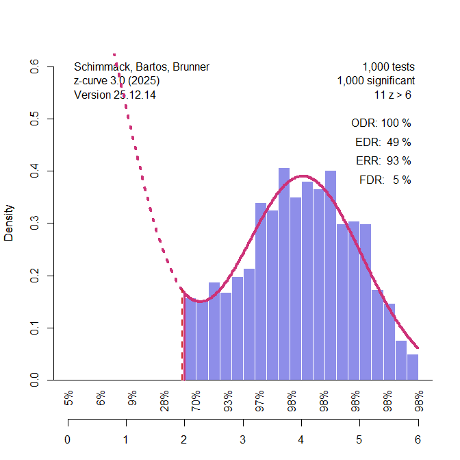
Z-curve was developed to evaluate the credibility of a set of statistically significant results. It operates on the distribution of significant test statistics and estimates quantities such as the expected replication rate (ERR), the expected discovery rate (EDR), and the false discovery rate (FDR). Its performance has been evaluated using extensive simulation studies covering hundreds of conditions that varied effect sizes, heterogeneity, and false positive rates.

A recent critique raised concerns about z-curve based on a simulation in which confidence intervals for the EDR showed low coverage. From this result, it was suggested that the method is unreliable (“concerns about z-curve“).

It is useful to examine carefully what this simulation does and how its results are interpreted.

Expected Values and Realized Data

The simulation assumes two types of studies: some that test true null hypotheses and others that test false null hypotheses with very high power. From this setup, one can compute expected values—for example, the expected number of false positives or the expected discovery rate.

Expected values, however, are averages over many hypothetical repetitions. In individual simulation runs, the realized number of false positives varies. In particular, when the expected number of false positives is close to one, it is common for some runs to contain no false positives among the significant results. In those runs, the observed significant record contains no false discoveries, and the realized false discovery rate for that record is exactly zero.

Evaluating coverage by comparing z-curve estimates to a fixed expected value in every run overlooks this variability. It treats a population-level expectation as if it were the true value for each realized dataset, even when the realized data are inconsistent with that expectation. This issue is most pronounced in near-boundary settings, where the quantities of interest are weakly identifiable from truncated data.

The simulation uses an extreme configuration to illustrate a potential limitation of z-curve. The setup assumes two populations of studies: one repeatedly tests a true null hypothesis (H0), and the other tests a false null hypothesis with very high power (approximately 98%, corresponding to z ≈ 4). Z-curve is applied only to statistically significant results, consistent with its intended use.

In the specific configuration, there are 25 tests of a true H0 and 75 tests of a false H0 with 98% power. From this design, one can compute expected values: on average, 25 × .05 = 1.25 false positives are expected, implying a false discovery rate of about 1.6% among significant results. However, these values are expectations across repeated samples; they are not fixed quantities that hold in every simulation run.

Because the expected number of false positives is close to one, sampling variability is substantial. In some runs, no false positive enters the set of significant results at all. In those runs, it is not an error if z-curve assigns zero weight to the null component and estimates an FDR of zero; that estimate matches the realized composition of the observed significant results.

When I reproduced the simulation and counted the number of false positives among the significant results, I found that the realized count ranged from 0 to 5, and that 152 out of 500 runs contained no false positives. This matters for interpreting coverage: comparing z-curve estimates in these runs to the expected false discovery rate of 1.6% treats a population-level expectation as if it were the true value for each realized dataset. As a result, the reported undercoverage is driven by a mismatch between the evaluation target and the realized data in a substantial subset of runs, rather than by a general failure of z-curve.

Reexamining Z-curve Performance with Extreme Mixtures

To examine z-curve’s performance with extreme mixtures of true and false H0, I ran a new simulation that sampled 5 significant results from tests of true H0 and 95 significant results from tests of false H0 with 98% power. I used a false positive rate of 5%, because a 5% false positive rate may be considered the boundary value for an acceptable error rate. Importantly, increasing it further would benefit z-curve because it becomes easier to detect the presence of low powered hypothesis tests.

As expected, the coverage of the EDR increased. In fact, it was just shy of the nominal level of 95%, 471/500 (94%). Thus, low coverage is limited to data with fewer than 5% false positive results. For example, the model may suggest no false positives, but the true false positive rate is 4%.

It is also possible to diagnose data that can create problems with coverage. First, a decreasing slope from significance to z = 3 implies a large number of missing non-significant results that can be identified by their influence on the distribution of significant z-values. In contrast a flat or positive slope suggests that high powered studies have a stronger influence on the distribution of z-values between 2 and 3. I computed the slope using the kernel density of the observed data and regressing the densities on the z-values. A positive slope perfectly predicted bad coverage, 29/29 (100%).

Another diagnostic is the ERR. A high ERR implies that most studies have high power and that there are few low powered studies with significant results to estimate the EDR. All failures occurred when the ERR was above 90%.

Finally, we can use the weights of the low powered components (z = 0, z = 1). When these weights are zero, it is possible that the model had problems estimating these components. In all failures, both weights were zero.

Importantly, these results also show that z-curve does not inevitably fail under this type of mixture. The issue is not the false positive rate per se, but the amount of information available to estimate it. With the same false positive rate of 5%, but a larger number of significant results—for example, 50 false positives out of 1,000—z-curve reliably detects the presence of missing non-significant results, even when the slope is increasing and the ERR is high. In this case, the weight of the z = 0 component was estimated at approximately 52%. By contrast, when the estimated weight is zero and the FDR estimate is zero, the true false discovery rate may still be as high as 5%, reflecting weak identifiability rather than estimator bias.

Conclusion

The low coverage reported in this simulation is largely an evaluation artifact. In this extreme setup, the expected false positive rate (about 1–2%) is an average across runs, but the realized number of false positives among significant results varies; in many runs it is zero. In those runs, the realized FDR is exactly zero, so an estimate of zero is not an error. Treating the expected rate as the “true value” in every run mechanically produces undercoverage.

When the false discovery rate is modest (e.g., 5%) and the number of significant results is larger, coverage is close to nominal and improves further as information increases. The remaining failures are confined to diagnostically identifiable cases in which high-powered studies dominate the significant z-values, leaving too little information to estimate the EDR.