You can find links to the other chapters on the post with Chapter 1.

The code for this chapter can be found on GitHub.
zcurve3.0/Tutorial.R.Script.Chapter9.R at main · UlrichSchimmack/zcurve3.0

This chapter examines the influence of one p-hacking method on z-curve (and p-curve) estimates of power (see Chapter 5 for a previous comparison of z-curve and p-curve). P-hacking is a term for statistical tricks that researchers can use to increase the probability of a significant result. This can be considered desirable when there is a true effect as a significant result avoids a so-called type-II error (failing to reject a false null-hypothesis). However, this argument ignores that p-hacking inflates effect size estimates and increases the risk of rejecting a true null-hypothesis. The replication crisis has shown that p-hacked results often do not replicate. The question is whether such replication failures can be predicted by z-curving p-hacked results.

Chapter 9: The Influence of P-Hacking V1.

There are different p-hacking methods, and they can have different effects on the distribution of z-values and z-curve estimates. It is therefore important to examine them one-by-one. The present study examines a method that was used by Bem (2011) to provide false evidence for time-reversed cognition (knowing something that has not yet happened or studying after an exam improves exam scores). To obtain significant results, he did two things. First, he checked whether studies showed promising trends and abandoned studies that failed to do so. Second, he combined smaller samples into one study (Letter to JPSP). This practice was considered acceptable by the editor of JPSP, implying that it may have been a common strategy to get significant results with low power (Kitayama). I call this approach patchwork sampling. This approach is also more efficient than a similar strategy called optional stopping. Optional stopping implies that researchers continue to collect data until they get a significant result. The problem with this strategy is that it can take many participants to reverse a negative trend in the beginning. It is much more efficient to abandon these samples and focus on samples with the desired trends.

Patchwork sampling is also consistent with the common claim among social psychologists that results are sensitive to small variation in experiments. How would they know this. Well, they do many small studies with small variations. When a study doesn’t show the desired result, the moderator is blamed, and the results can be ignored. However, if two studies show the same trend, the moderator can be ignored, and they can be combined to produce p < .05.

The present simulation assumed that researchers conduct up to three studies with small samples. A significant result in a small sample is reported. If they are not significant, two samples are combined which produces another 3 chances to get p < .05. If that fails, all three samples are combined for another test. If none of the tests produce a significant result, the results are not reported.

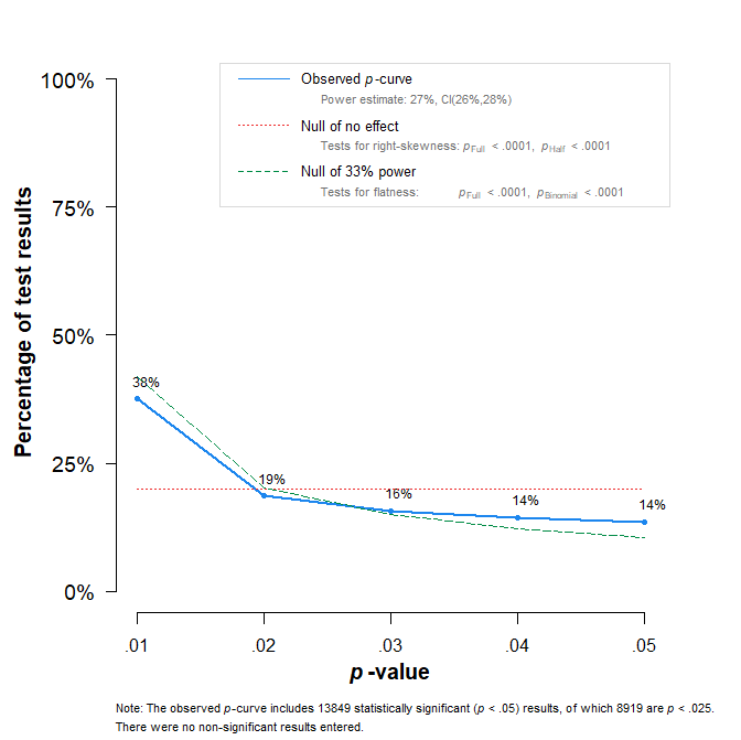
P-hacking differs from simple selection bias. it is often assumed that p-hacking can be detected with p-curve analyses (Figure 1). A p-curve plot shows the distribution of p-values between 0 and .05. Without a real effect and without p-hacking there are equal frequencies of p-values in the bins from 0 to .01, .01 to .02, … .04 to .05. Some p-hacking methods will produce more p-values close to .05 than .01. This is called a “left-skewed” distribution. Figure 1 shows that p-curve detects patchwork sampling when the studies test a true null-hypothesis (no effect).

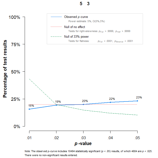
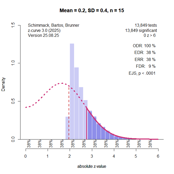
It is often overlooked that p-curve does not detect p-hacking when the studies test a true effect even if the effect is small and power is low. Figure 2 shows the p-curve plot with mean effect size d = .2, SD of effect sizes = .4, and n = 15 per group. The simulated data are p-hacked, but the p-curve plot fails to detect p-hacking.

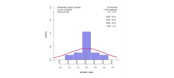
Z-curve 3.0 uses a different approach to detect p-hacking methods that produce too many p-values close to .05. It is possible to fit z-curve to any set of z-values. To test for p-hacking, z-curve is fitted to z-values greater than 2.8 (p = .005). The model then predicts the distribution of z-values in the range between 1.96 (p = .05) and 2.8 (p = .005), and the observed frequency of z-values in this range can be compared to the predicted frequency.

Figure 3 shows the results for the same simulation that was used for the p-curve in Figure 2. The figure shows that there are many more observed (purple bars) than expected (dotted red line) values between 2 and 2.8.

The simulations examine the type-I and type-II error rates of this approach to the detection of p-hacking.

The Simulation

The simulation varied cell sizes of a two-group design (n = 15, 20, 30), effect sizes (0 to 1 in steps of .2) and heterogeneity in effect sizes with standard deviations of 0, .2, .4, .6, and .8. This covers common ranges of heterogeneity in meta-analyses. Each study was run to have 10,000 successful attempts to get at least one significant result for every attempt. The actual number of significant results could be higher when power was high because more than 1 of the 7 attempts could produce a significant result.

The data were analyzed once without p-hacking using the results of the three small samples and once with p-hacking. The simulation without p-hacking was used to estimate the type-I error of the p-hacking bias test. The other simulations were used to examine the influence of p-hacking on z-curve estimates and to estimate the type-II error of the p-hacking bias test. Z-curve was fitted once with the default method that does not make distribution assumptions and once with a single component that assumed a normal distribution of power.

Results

Inflation of Success Rates

P-hacking increases success rates. When the null-hypothesis is true, the inflation of the success rates increases the risk of a type-I error (a false rejection of the null-hypothesis). However, when there is a true average effect, p-hacking essentially increases power to reject a false null-hypothesis. The problem is that we do not know whether the null-hypothesis is true or false. Thus, p-hacking is risky and invalidates the assurance that no more than 5% of tests can falsely reject the null-hypothesis.

Figure 4 shows how much the patchwork method simulated here inflated success rates.

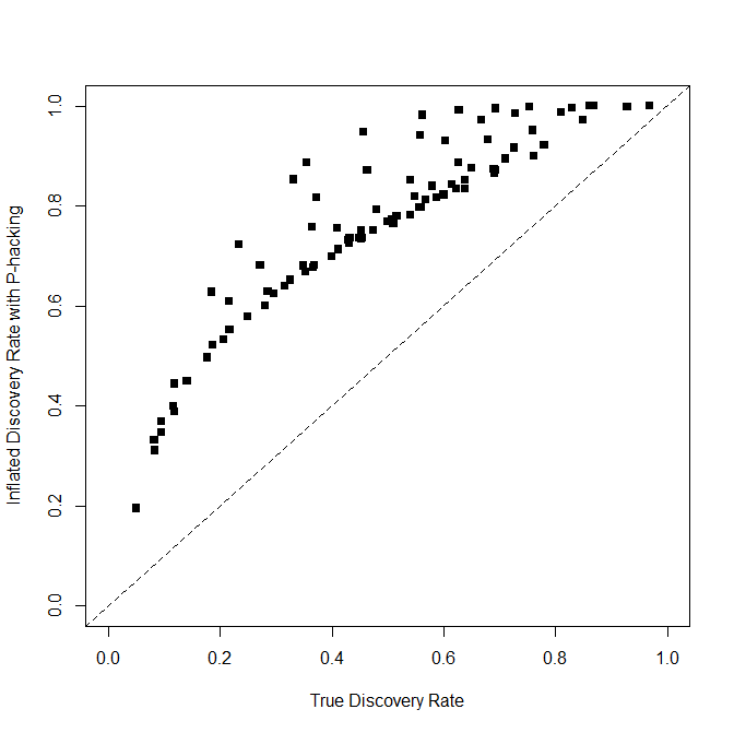
This p-hacking method boosted the success rate from 5% to 19% when the null-hypothesis was true. On average, it increased power to detect a real effect by 28%, but the figure shows that the amount depends on the real power. With low power and real effects, success rates are inflated by up to 50%. This does not justify p-hacking, but it does show the appeal to use p-hacking.

P-Hacking Bias Test

The p-hacking bias test was significant in 9 out of 90 (10%) simulations for the default method and 12 out of 90 (13%) for the normal z-curve. In the simulations with bias, the default method had 52 out of 90 (58%) significant results and the normal z-curve had 74 out of 90 (82%) significant results. Importantly, these success rates were obtained with very large samples. In short, the p-hacking bias test is promising, but non-significant results do not imply that there is no bias. Thus, it is important to examine how p-hacking influence z-curve estimates.

Z-curve Estimates of the Expected Replication Rate (ERR)

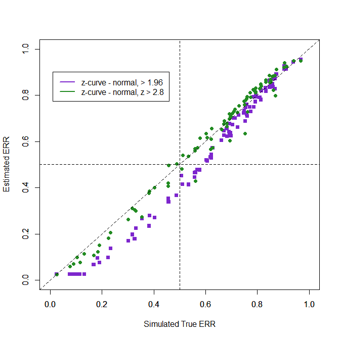
Overall performance of estimation methods can be examined with the root mean square error (RMSE) where error is simply the difference between the simulated true ERR and the z-curve estimate. There are four z-curve estimates using default and normal models and using all significant values or only z-values greater than 2.8 to avoid bias from p-hacked just significant results.

Method……………………..RMSE
Z-curve default – all….. .075
Z-curve normal, all ….. .070
Z-curve default, >2.8… .064
Z-curve normal, >2.8 … .035

The results are similar, but the normal method works better because the simulation used normal distributions of effect sizes. Also, excluding the p-hacked just-significant results produced better results.

.
The figure shows the superior performance when just significant results are excluded. Even if the bias test is not significant, excluding just-significant results may be useful to reduce the influence of p-hacking or at least to examine the robustness of results.

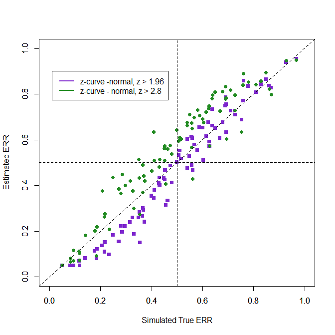
Z-curve Estimates of the Expected Discovery Rate (EDR)

Estimating the distribution of all z-values from the distribution of only significant results (or only z > 2.8) is difficult, especially when p-hacking is used. Nevertheless, the RMSE values show some accuracy. The normal model outperforms the default method because it is easy to predict the missing values from a truncated normal model. This works in these simulations because the assumption fits the simulated data. However, using only z-values greater 2.8 does not improve performance because extreme values provide less information about the distribution of non-significant z-values.

Method……………………..RMSE
Z-curve default – all….. .146
Z-curve normal, all ….. .066
Z-curve default, >2.8… .180
Z-curve normal, >2.8 … .096

Using only z-values greater than 2.8 leads to overestimation of the EDR.

One way to examine the possible influence of patching samples would be to conduct analysis for subsets of studies with different sample sizes. In the present case, the smaller samples will produce stronger estimates because they are not p-hacked than the p-hacked larger samples. If this is the case, the results from the smaller samples could be used.

Conclusion

P-hacking creates a problem for selection models that simply assume non-significant results are not reported because p-hacking changes the distribution of test-statistics and it is not known which p-hacking methods were used. This simulation examined one method that leads to underestimation of the ERR and EDR. The p-hacking bias is difficult to detect and also difficult to correct. At present, my recommendation is to compare results across different models (sensitivity analysis), but to focus on the results with the default method. The underestimation of EDR and ERR can be considered a penalty for p-hacking that creates an incentive to avoid p-hacking. In the present scenario, researchers are conducting many small studies. If a real effect is present, they could present all studies, including non-significant ones, with a meta-analysis of the studies or combine the studies into a single dataset. In contrast, not publishing the non-significant results to present a perfect picture of only successes undermines the credibility of the published results (Schimmack, 2012).