You can find links to the other chapters on the post with Chapter 1.

The code for this chapter can be found on GitHub.
zcurve3.0/Tutorial.R.Script.Chapter8.R at main · UlrichSchimmack/zcurve3.0

This chapter compares different transformations of t-values into z-values to be analyzed with z-curve. Only t-values are considered because F-values from studies with one experimenter degree of freedom can be converted into t-values, t = sqrt(F). Chi-square tests with one degree of freedom can be converted into z-scores, z = squrt(chi-square). Test-statistics with more complex designs are rare and do not test a clear hypothesis. They require follow up tests to determine the pattern and the follow-up tests can be used.

Chapter 8: From t-values to z-values

The t-distribution was discovered in 1908 by William Sealy Gosset, a statistician at the Guinness Brewery in Dublin. It is useful when the population standard deviation is not known, and sample sizes are small. Ronald A. Fisher later formalized its use within the framework of hypothesis testing and many comparisons of two groups or correlations rely on t-distribution for significance testing.

The problem for meta-analysis is that studies with different sample sizes have different distributions. A value of 2 is significant, p < .05, two-sided, with the normal distribution and in large sample sizes, but not in small sample sizes. Z-curve requires that all test-values are comparable and have the same sampling distributions. Therefore t-values need to be transformed into z-values. This approximation can introduce biases in z-curve results if sample sizes are small. The question is how big these biases are and how this bias can be minimized.

This blog post examines four methods to use t-values with z-curve.

1. The default method in z-curve is to use two-sided p-values and convert them into z-values. This approach is useful because it does not require information about the degrees of freedom.

2. Another approach that is often used in literatures with large sample sizes is to simply ignore the degrees of freedom and use the t-values as if they are z-values. z = t. The main problem of this approach is that t-values increasingly overestimate power as degrees of freedom decrease.

3. The third method is new and was developed for z-curve.3.0. Rather than computing the p-value under the null-hypothesis for all t-values, the method uses the mean of the t-values to pick the non-centrality parameter for the transformation. With low means, it uses a value of 0 and there is no difference to the p-value method. With moderate means, it uses a moderate non-centrality parameter around 2. For high means, it uses a high non-centrality parameter around 4. This changes the transformation distribution in accordance with the typical distribution of the observed t-values.

4. The fourth method uses the t-distribution to model the observed t-values. This method is essentially a z-curve with t-distributions and can be called t-curve. It is now implemented in z-curve 3.0 and can be used by supplying a fixed df value and requesting the estimation method “DF.” This method is useful when all studies have small df (N < 30), and because df cannot be less than 1, df of studies with small samples have a relatively small range with similar distributions.

The illustration first shows the effect of degrees of freedom on the t-distribution when power is 50%. Figure 1 shows the results for studies with N = 100 (df = 98 for a two-group comparison). The distributions are not identical, but very similar and have little influence on z-curve estimates.

.

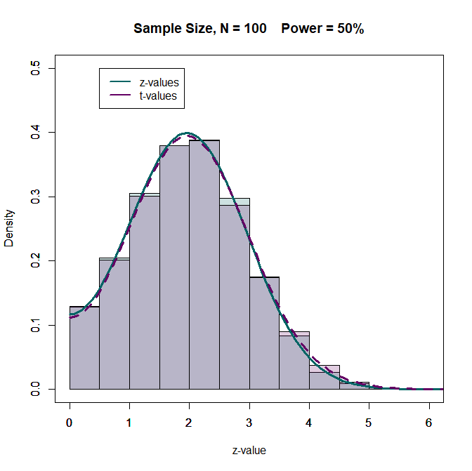
What happens when sample sizes are smaller. In the (not so good) old days, sample sizes were often n = 20 per group. This gives a total sample size of N = 40 and 38 degrees of freedom. However, sometimes some values are missing. Let us examine a scenario with N = 30. The distributions are still fairly similar. How do these small differences influence z-curve estimates?

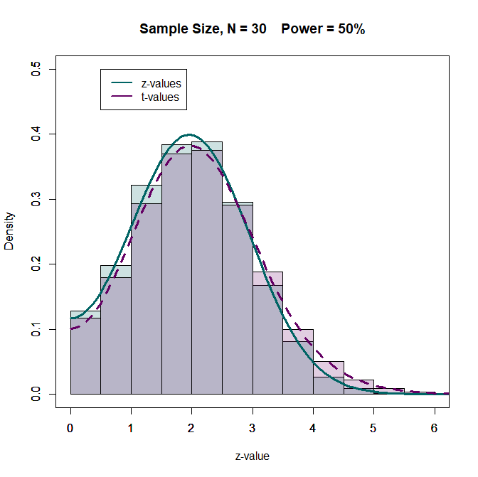
The z-curve estimates for the z-values are within 1 percentage point of the true values.

The z-curve estimates based on the t-values are slightly inflated and the difference is 5 percentage points for the ERR. The results for other levels of power are similar (see simulation results below).

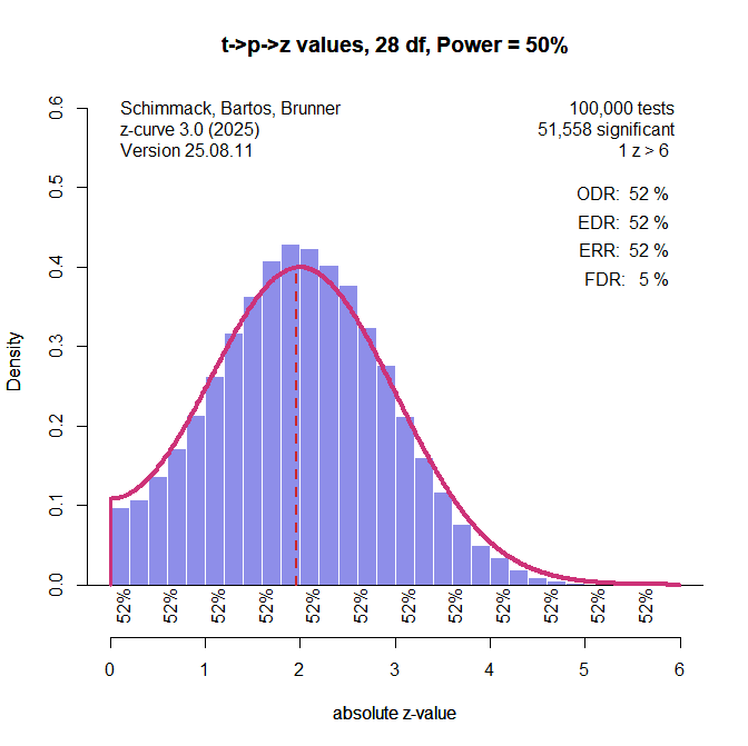
The next figure shows the results for t-values converted into p-values and then converting p-values into z-values. This procedure does not produce z-values and the distribution is slightly different than the distribution for actual z-values, but the transformation produces slightly better estimates than the use of t-values as z-values.

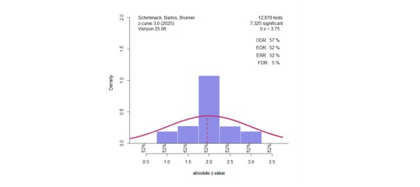
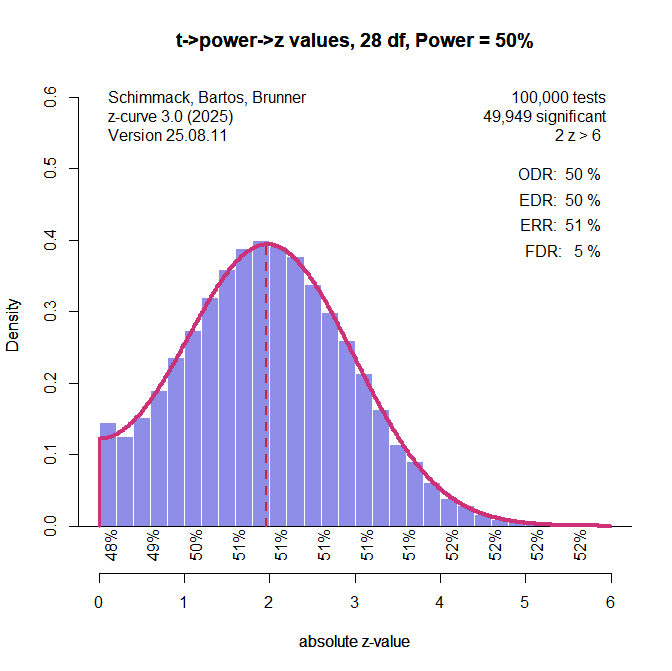
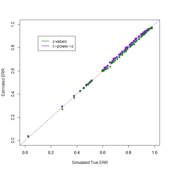
The next figure shows the results using conversion of t-values to power and then converting power to z-values. With a median of the significant t-values of 2.8, a value of 50% power is used for the transformation. This produces perfect estimates when power is indeed 50%. Some bias will be introduced when the power of the transformation does not match the true power. The extend of this bias will be examined in the simulation study. The illustration shows that using p-values or power is not identical because the t-distribution differs for different non-central t-values.

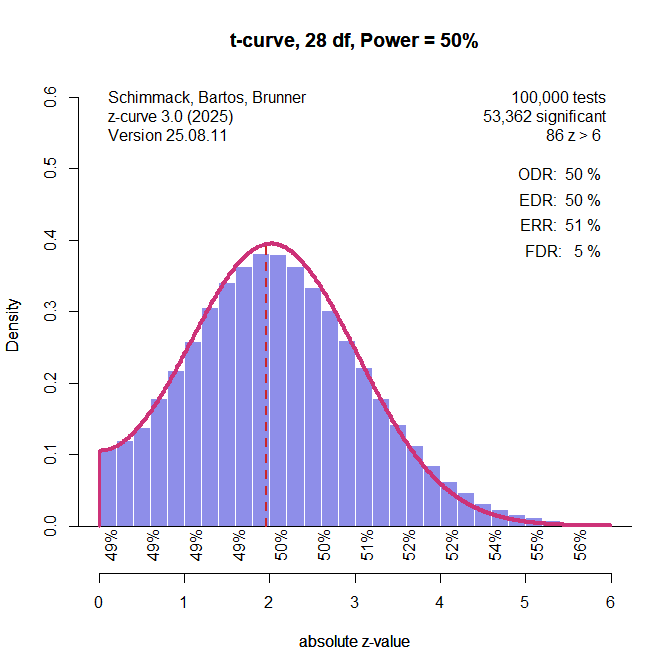
Finally, I added a t-curve option to z-curve.3.0. Users can provide a df-value and request fitting t-distributions with the specified df-value to the data. When all studies have the same df, the model fits perfectly.

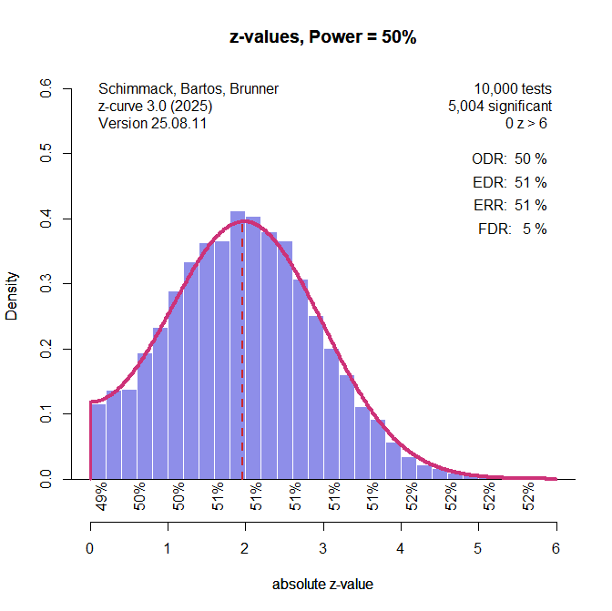
The illustrations used all observed data, but z-curve was developed for datasets with selection bias. The simulations examine the performance of the different methods when only significant results can be used and z-curve estimates the average (unconditional) power of the studies with significant results (i.e., the expected replication rate, ERR), and extrapolates from this distribution to estimate the full distribution, including the missing non-significant results. The average power of all studies is the expected discovery rate (EDR) that predicts how many significant results researchers actually observed when they analyzed their data. When the EDR is lower than the observed discovery rate (i.e., the percentage of reported significant results), we have evidence of publication bias.

The Simulation

The setup of the simulation study is described in more detail in Chapter 4. The most important information is that the original studies are assumed to be mixtures of three normal distributions centered at 0, 2, and 4. To obtain t-values, the z–values are converted into power (loosely speaking, for 0 the value is 0 and H0 is true and power* is alpha). The power for z2 is 50% and the power for z4 is 98%. With weights ranging from 0 to 1 in 0.1 steps, we get 66 unique mixtures of the three components. The simulation simulates large sets of studies, k = 100,000 to minimize random sampling error and reveal systematic biases in the different estimation methods. The simulation uses only significant results to see the performance of the transformation methods when selection bias is present.

Results

Expected Replication Rate

The expected replication rate is the average probability of studies with significant results to produce a significant result again in an exact replication study. To compare the estimates of the ERR, I computed the root mean square error (RMSE). A value of .01 implies that estimates are on average within 1 percentage point of the true value.

Method RMSE
1. z-values………….. .005
2. t-values …. ……… .081
3. t -> p -> z ..,,…….. .026
4. t -> power -> z…. .011
5. t-curve …………… .005

The results show that the use of t-values as if they were z-values is inferior to other methods. The default approach to convert t-values into p-values and the p-values into z-values works better, but the new methods work even better. Not surprisingly, analyzing t-values with 28 degrees of freedom with a model that fits this assumption works as well as analyzing normal distributions with z-curve that assumes normal distributions of sampling error.

The next figure examines the performance of the methods visually using the results for z-values as a standard of comparison.

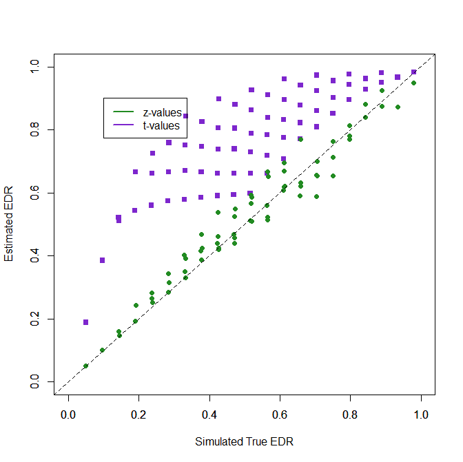
1. Using t-values as z-values

2. Default transformation in z-curve 1.0 and 2.0

Using t-values as if they were z-values leads to overestimation of power because t-values are larger than z-values. More interesting is that the bias is more pronounced for lower levels of power. When the null-hypothesis is true, t-values estimate 20% power, a very misleading result.

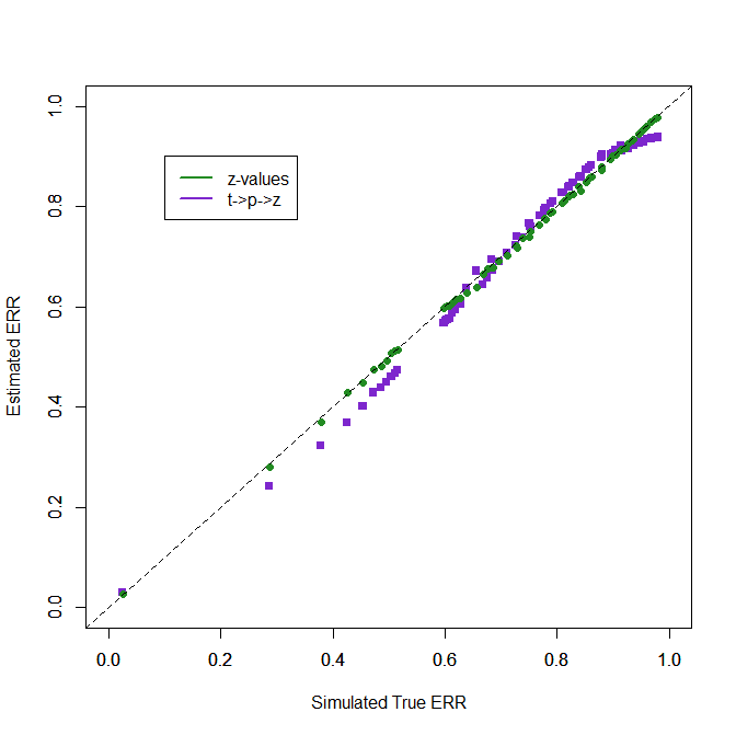
The default method does not have this problem. It can identify sets of studies with only false positive results. It shows the opposite trend to underestimate power for moderate levels of power, but the bias is small and not practically relevant. It does well for moderate to high power and only shows a small trend to underestimate again close to the maximum probability of 1. Overall, these results show that the default transformation of t-values into z-values that has been used in published articles works reasonably well even if sample sizes are as small as N = 30. As most studies have larger samples sizes and bias is even smaller, the approximation of t-values with z-values does not undermine the validity of z-curve results. This confirms earlier findings with simulations that used t-values and typical sample sizes from psychology (Bartos & Schimmack, 2022; Brunner & Schimmack; 2020). Remember that these results also generalize to F-tests with 1-experimenter degree of freedom because these F-values are just squared t-values.

3. Transformation with (Unconditional) Power

However, some areas in psychology have even smaller sample sizes than N = 30, and the bias of the default method gets larger. In these situations, users of z-curve can use one of the two new methods. The first approach uses the probability of a significant result (loosely called power) to convert t-values into z-values. The probability is chosen based on the median t-value of the significant results. When it is low, a probability of 5% is used and the conversion is like the p-value conversion. When the median significant t-value is moderate, a probability of 50% is used and the non-central t-value and z-value that produce this probability is used. When the median significant t-value is high, a probability of 75% and the corresponding non-central z and t-values are used. The specific values are not relevant. What is important is that the t-distribution approximates the distribution of the true distributions better when the non-central values are closer to the actual ones. The figure shows that this method performs as well as z-curve analysis with true z-values for the full range of ERRs.

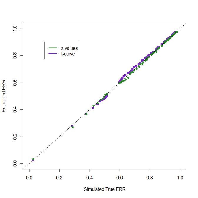
4. Analyzing t-values with t-curve

The t-curve option simply fits the mixture model of z-curve using t-distributions with a fixed df for all studies. It does as well as z-curve with z-values and does not require a conversion of test-statistics. Thus, it is the preferred method to estimate ERR for sets of studies with small df.

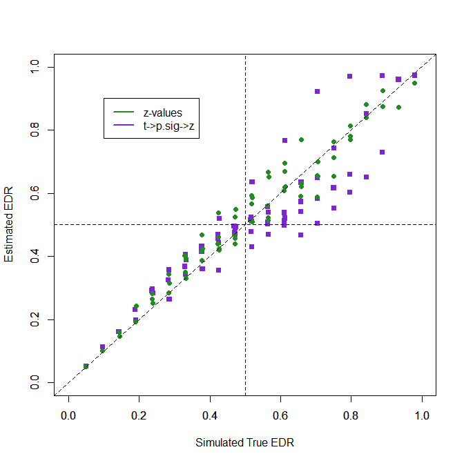
Expected Discovery Rate

The expected discovery rate (ERR) is the average probability of all studies to produce a significant result, including studies with non-significant results. As non-significant results are not observed due to simulated publication bias, z-curve has to guess the distribution of non-significant results from the distribution of significant results. This leads to more uncertainty and more room for bias in EDR estimates and the RMSE values are larger than the RMSE values for the ERR. The question is only how transformation methods compare to the estimates based on z-values.

Method RMSE
1. z-values…………. .049
2. t-values … ……… .280
3. t -> p -> z ..,,……. .165
4. t -> power -> z…. .090
5. t-curve …………… .057

Three patterns in the RMSE results are noteworthy. First, the default transformation introduces considerable bias in the estimation of the EDR. Second, the new transformation using differnet levels of unconditional power is a notable improvement. Finally, analyzing t-values with t-curve also is notably better than using transformations. Why t-curve with t-values shows slightly worse fit than z-curve with z-values is not clear at this moment, but the difference is minor and using the t-curve option is recommended if all or most studies are small.

1. Using t-values as z-values

No comment.

2. Default transformation in z-curve 1.0 and 2.0

Some comments are required for the default method. First, the plot is ugly, but remember it is based on a sample size of 30. So, it merely shows that the default method should not be used when most studies are small which has not been the case in actual applications of z-curve to real data.

Second, the biggest problem is that z-curve overestimates the EDR when the true EDR is high. The reason is that it can be tricky to detect that the published studies with high power were obtained from also testing a large number of studies with low power that produce few significant results and are not “published.”

From a practical point of view, this is not a big problem. Say researchers conduct 4 small pilot studies with low power. They publish these pilot results when they produce a significant result, but do not report them when they do not. Then they conduct a more powerful study that is more likely to produce a significant result. Omitting the small pilot studies with non-significant results does not distort the literature. The real problem remains that the larger more powerful study is not reported if it also does not produce a significant result. This is revealed by the ERR. In real datasets, these patterns are rare and most z-curves show a mode (peak) at 1.96 rather than at 4.

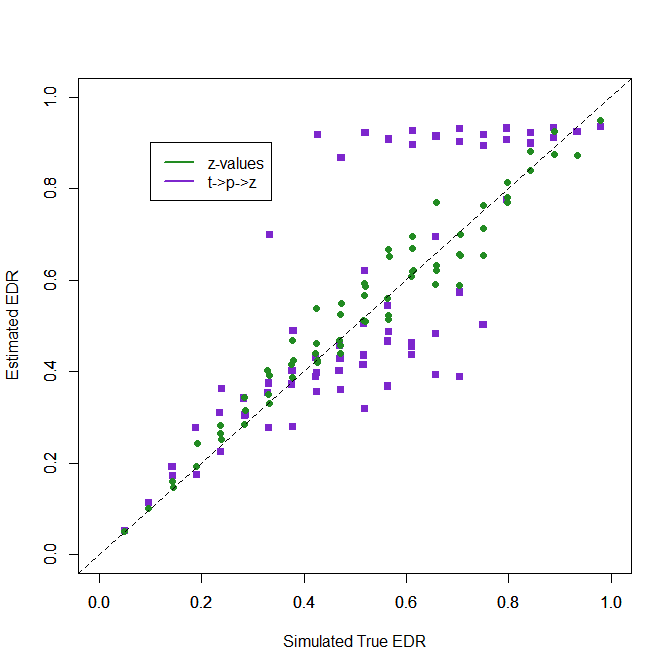
3. Transformation with (Unconditional) Power

The new transformation using unconditional power works better because it does a better transformation for large t-values. The key problem that remains is that moderate ERRs in the 50-70% range are underestimated, but most true EDRs over 50% are estimated to be over 50%, and those below 50% are estimated to be below 50%. The transformation is used when most studies have larger sample sizes. So, the bias seen here is reduced by the percentage of studies with small sample sizes.

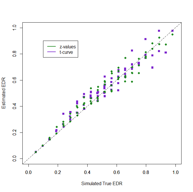
4. Analyzing t-values with t-curve

When all studies have small df, the new t-curve method can be used. The results for t-curve with t-values and z-values with z-curve are difficult to distinguish. There appears to be a bit more variability for really high values. Nevertheless, these results provide the first validation evidence for the use of t-curve. The good performance of t-curve is of course expected. All models work well when simulated data meet the assumptions of the model. Further validation research needs to examine how well t-curve works when small studies have different sample sizes. With really small df (df < 5) the method may not work well, but then, why not collect data from 3 more participants or just do a replication study with twice the sample size (N = 10)? (LOL).

Conclusion

Z-curve uses transformation to z-values to model sampling distributions of different statistical tests. This can introduce bias because sampling distributions of other tests differ from actual z-tests. Here I examined how much bias different transformations produce and presented a new transformation method that works better than the default method used in z-curve 1.0 and 2.0. I also showed that data from small samples can be better analyzed using actual t-distributions and demonstrated the performance of the new t-curve option. The results address concerns that z-curve estimates are not trustworthy because each test has a different sampling distribution. This broad criticism is not valid because differences between t-distributions and the standard normal are trivial once we reach even modest sample sizes of N = 100. Even for sample sizes of 30, the transformation introduces only small bias for the ERR and EDR estimates are still useful. Users of z-curve need to be aware of the possibility of bias, but they can be confident that z-curve produces useful estimates of (unconditional) power that can be used to estimate expected discovery and replication rates.