You can find links to the other chapters on the post with Chapter 1.

This chapter compares z-curve 3.0 to the Bacon mixture model using both unbiased replication data and a 66-scenario simulation study. We evaluate accuracy for key meta-analytic metrics (EDR, ERR) under varying heterogeneity conditions. The results show that the default z-curve method performs better than the Bacon mixture model. The chapter explains why z-curve is performing better.

Chapter 7: Z-Curve with Bacon

Z-curve is one of the few mixture models that model selection bias. Many mixture models have been developed to analyze significant and non-significant z-values under the assumption that there is no selection bias. This assumption makes these models not very useful for meta-analysis of published results because selection bias can distort these results. Nevertheless, it is interesting to compare these mixture models with z-curve.

Z-curve was specified in four different ways using the density approach. First, the default model with seven components (ncz = 0, 1, 2, 3, 4, 5, 6) was used. Second, a model with three components with free population means and fixed SD of 1 was used. Third, a model with two components with free population means and standard deviations was used. This is a frequentist alternative to the Bayesian bacon mixture model.

The population means, population standard deviations, and weights were used to compute the expected discovery rate (EDR). This is the average power of all studies with non-significant and significant results. Computing this probability is not really useful because it matches the percentage of significant results without selection bias. So, we are not learning anything new from the estimate of average power. Here, the results help us to evaluate the performance of the different mixture models.

The code for this chapter can be found on GitHub.
zcurve3.0/Tutorial.R.Script.Chapter7.R at main · UlrichSchimmack/zcurve3.0

Illustration With Open Science Collaboration Data

A one component model with a normal distribution runs into problems when the true distribution is not normal. In a simulation with just three components centered at 0, 2, and 4 this happens when we have 50% of studies with z = 0 (the null hypothesis is true) and 50% of studies have high power (z = 4, power = 98%).

For a two-component model like bacon this is not a problem. It can fit this scenario with two components that have means of 0 and 4 and standard deviations for the sampling error of 1 .

The real problem for models with two components and normal distributions is that real data often have a long tail of studies with large z-values (z > 6). Models like p-curve cannot handle these long tails and lead to largely inflated estimates of power (see Chapter 5). Z-curve solves this problem by fitting the model to z-values below 6 and assigning a power of 1 to z-values greater than 6. Remember, even a z-value of 4 already has 98% power.

I am using the data from the replication studies of the reproducibility project (Open Science Collaboration, 2015) to illustrate z-curve and bacon (see Chapter 3 for a detailed examination of these data with z-curve). The advantage of using the replication data is that they have no publication bias.

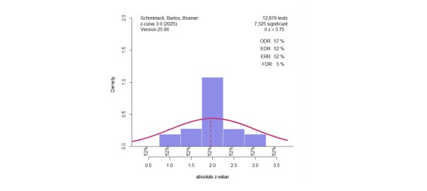
Figure 1 shows the results with the default model with seven components and fixed variances of the sampling error at 1. I used the density method to make the results more comparable.

the results confirm that there is no publication bias. The observed discovery rate (% of significant results) is 33% and the z-curve model estimate of the expected discovery rate is 33%. The fitted line matches the histogram fairly well. The expected replication rate is 74%. That is, 74% of the studies that were successfully replicated are expected to be significant again in a second replication attempt. Based on the EDR of 33%, we can estimate the false discovery risk (FDR); that is, the maximum percentage of significant results that could still be false positive results. The FDR is 11%.

Figure 2 shows the results for a model with three components with free means and SD = 1. The results within 2 percentage points of the previous results and the EDR is overestimated by 1 percentage point. This shows how flexible mixture models are. They can fit data even if the model does not match the data generation model. The means and SD of the components are not interpretable, but they can be used to estimate average power (Brunner & Schimmack, 2020).

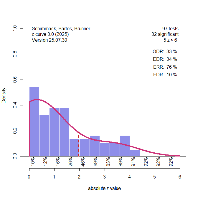
Figure 3 shows the results for a model with two components with free means and SDs. These results are directly comparable to the results for the bacon model which also uses two free components, but with a Bayesian estimation method. The results with the z-curve density method are similar to the previous results. This shows that a model with two free components is flexible enough to approximate the distribution of these data.

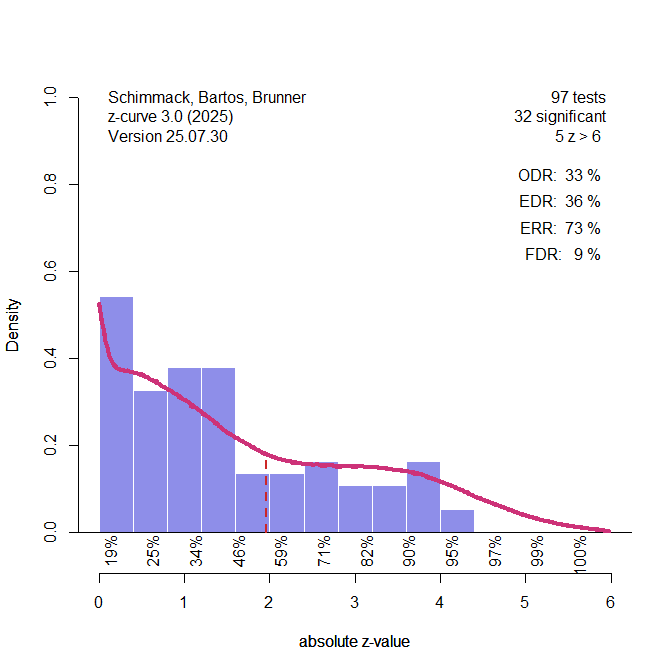
Figure 4 shows the results for the bacon model. Here the bacon model was used to fit the data and the estimated weights, means, and standard deviations were used as fixed values for the z-curve model. Importantly, the z-curve method did treat the 5 extreme values (z > 5) as studies with 100% power.

The bacon model assigned a weight of .04 to negative population means. The weight, mean and, standard deviation of the first component were w = .82, M = 0.06 and SD = 1.21. The weight for the positive component was .14. The standard interpretation of these results would be that only 14% of these results have a true effect in the predicted direction.

When we use the components to estimate a z-curve, we see similar results to the analysis with the z-curve density method. We also see that the false positive risk for significant results is 9%. With 33% significant results, this suggests that 33*(1 – .09) = 30% of the results are true positive results. This estimate is higher than we would predict based on the bacon method, 14%.

The problem with the 14% estimate is that it is based on a realistic interpretation of the components. However, some studies with z-values close to zero may have tested a true positive result with low power. The z-curve method to estimate the false positive risk avoids this problem.

Figure 5 shows the bacon results without truncating z-values at 6. Although there are only 5 z-values greater than 6, the bacon estimate now underestimates the EDR and ERR because a model that assumes a normal distribution does not capture the tail of extreme values. The low estimate of the EDR also implies an inflated estimate of the false discovery risk.

In conclusion, the frequentist z-curve method without priors performs as well or better than the Bayesian bacon method with priors. Moreover, the assumptions of the bacon mixture model that there are only two components limits its ability to fit data with a long tail of strong findings. This problem can be fixed by excluding the tail from the range of values that are fitted by the model, but there is no need to fix bacon because z-curve performs well.

The Simulation

The setup of the simulation study is described in more detail in Chapter 4. The most important information is that the original studies are assumed to be z-tests with three levels of power. Z0 assumes the test of true null-hypothesis with a center of the z-distribution at 0. This produces a power to replicate a study with p < .05 (two-sided) with an effect in the same direct. Z2 simulated a distribution centered at 2, slightly above the critical value for a significant result, z= 1.96. This is moderate power, slightly above 50%. The third component, Z4 is centered at a value of 4, and power is 98%. The mixture of these three components produces sets of studies with average power that covers the full range of power with few extreme values (z > 6) that might be considered outliers and are not used for the fitting of z-curve. The simulation program samples from the three distributions. To examine systematic biases, the simulation created 10,000 significant z-values. These simulations do not have a tail of extreme values and make it possible for bacon to perform as well or better than z-curve.

Results

Expected Discovery Rate

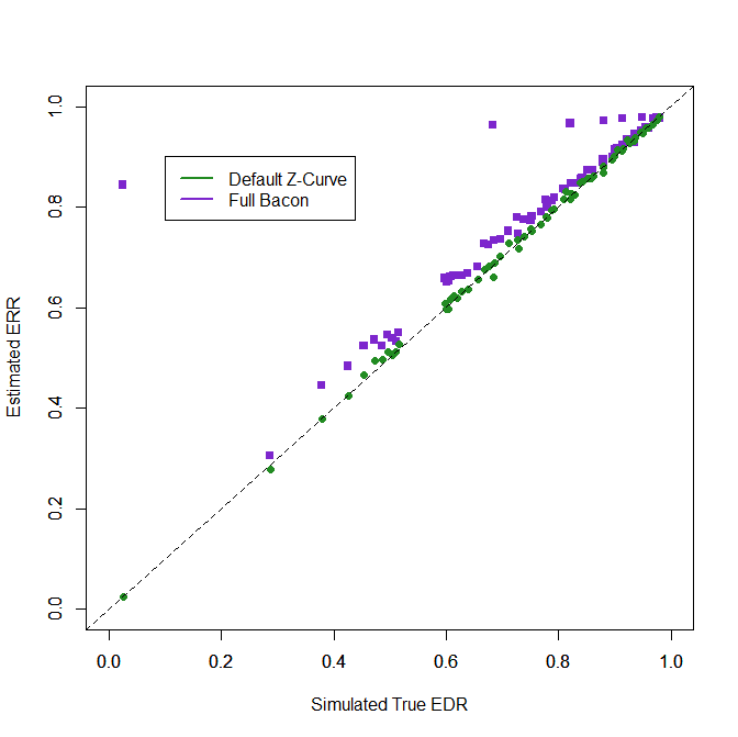
To compare the overall performance of all five models, I computed the root mean square error (RMSE). A value of .01 implies that estimates are on average within 1 percentage point of the true value.

RMSE
1. Default z-curve : .007
2. Three components : .007
3. Two components : .012
4. truncated bacon : .013
5. full bacon : .015

Figure 6 visually compares the default z-curve method with the full bacon method.

Both models produce good estimates, but these estimates are not useful in real data because we can simply compute the percentage of significant results to estimate average power. This method produces smaller confidence intervals and makes fewer assumptions. The only problem is that it assumes no publication bias, but that is also true for bacon.

Expected Replication Rate

The default z-curve method and the three-component model work well. The two-component model z-curve model is better than the truncated bacon model and the truncated bacon model is better than the full bacon model.

RMSE
1. Default z-curve : .007
2. Three components : .010
3. Two components : .018
4. truncated bacon : .034
5. full bacon : .011

Conclusion

This chapter compared z-curve to another mixture model that is being used to analyze data with a large number of statistical tests in large samples. The results show that z-curve performs better than this model because a model with two normal components does not capture the distribution of real data well, especially when they have a long tail of strong results. Brunner and Schimmack (2020) avoided this problem by excluding the tail of extreme z-values from the range of values to be fitted by the model. This does not mean that these values are ignored. Rather extreme values have little bias and high power. Thus, we can simply adjust the model estimates by making the assumption that the studies in the long tail have 100% power.

The bacon method is also not very useful for applied research purposes. First, we do not need to estimate the EDR without publication bias because we can simply compute the percentage of significant results to get an estimate of average power. This estimate can then be used to estimate the false discovery risk. The whole point of creating z-curve was to estimate power when publication bias is present. Z-curve is one of the few methods that have been developed and validated to detect and correct for publication bias. Another method was introduced earlier by Jager and Leek (2013), but Schimmack and Bartos showed with simulation studies that z-curve performs better. Therefore, z-curve is currently the best method when publication bias is present.