You can find links to the other chapters on the post with Chapter 1.

Chapter 6 compares the default z-curve to an alternative method that models heterogeneity with a normal distribution. The assumption of a normal distribution would make the model simpler and provide tighter confidence intervals. The drawback is that the distribution of power across studies may not be normal. A model that does allow for different distribution patterns performs better in these situations (Brunner & Schimmack, 2020).

zcurve3.0/Tutorial.R.Script.Chapter6.R at main · UlrichSchimmack/zcurve3.0

Introduction to Chapter 6

I assume that you are familiar with z-curve. Chapter 4 illustrated how z-curve models heterogeneity of power with mixtures of standard normal distributions. This allows z-curve to estimate average power without making assumptions about the distribution of power. Other meta-analytic methods often make assumptions about the distribution of power or effect sizes (Brunner & Schimmack, 2020). For example, the random effects selection model implemented in the R-package weightr assumes that effect sizes are normally distributed. This is an unrealistic assumption, but it may produce reasonable results in some settings. Simulation studies can help to examine under which conditions distribution assumptions work or do not work.

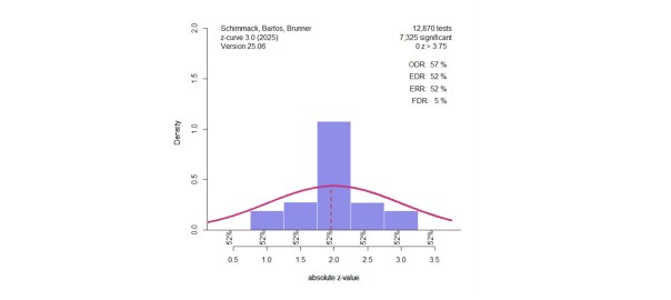
Here are two examples. The first example assumes that the average power of studies is 50%. This corresponds to a non-central z-value of 1.96. Sampling error would produce a normal distribution of observed z-values. Now let’s assume that studies vary in power with a normal distribution with a standard deviation of .5. This would mean 95% of the true power values range from 17% for a z-value of 1 to 85% for a z-value of 3. This is not an unreasonable assumption (Cohen, 1962).

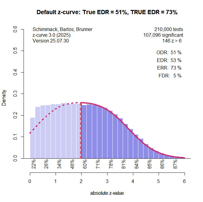
The default z-curve method provides a good estimate of the expected replication rate within 1 percentage point of the true value. The expected discovery rate is underestimated by 5 percentage points. As Figure 1 shows, it overestimates the amount of non-significant results.

Figure 2 shows the results for the z-curve that assumes a normal distribution and estimates the mean and standard deviation of this distribution. The true values are a mean of 2 and a standard deviation of the observed z-scores of 1.12. The estimated values are 1.97 and 1.13. It also produces good estimates of the EDR and ERR.

So, should we use this method. Yes, if we know that the distribution of the non-central z-values is normal. The problem is that we do not know the distribution in real data. So, what happens if we assume a normal distribution, but the actual distribution is not normal?

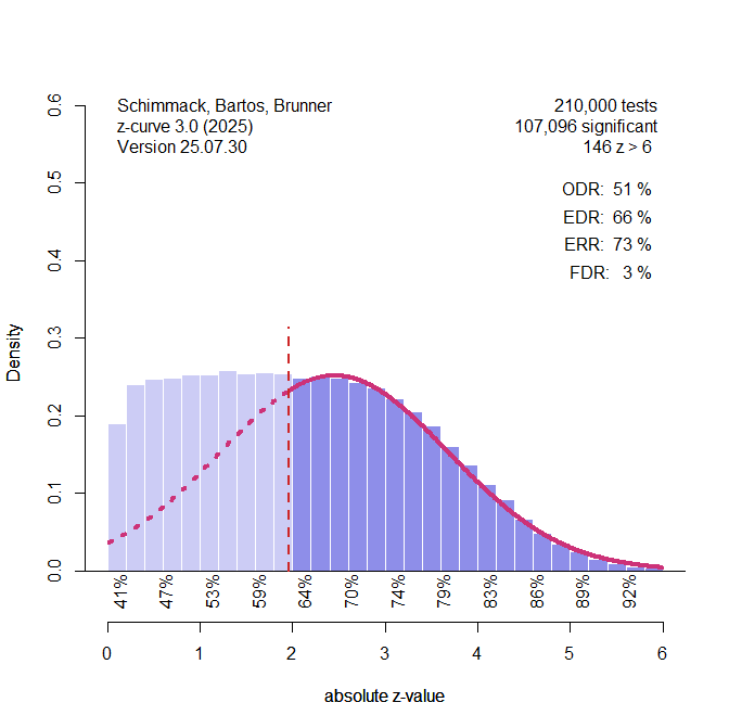
In this simulation there were 47.5% studies with ncz = 1, 5% studies with ncz = 2, and 47.5% studies with ncz = 3. The average is again 2, and power is in a range from ~20% to 85%, but the distribution is not normal.

Default z-curve handles this scenario well and estimates the distribution of the missing non-significant results pretty well. The EDR is overestimated by 2 percentage points.

This time, the model that assumes a normal distribution is biased. The assumption of a normal distribution leads to an underestimation of non-significant results that stem from the large number of studies with ncz = 1. As a result, the EDR is overestimated by 15%.

Two scenarios are not sufficient to evaluate the general performance of a model. I used the simulation study of Chapter 4 to evaluate the performance of the model that assumes a normal distribution of non-central z-values (NDIST z-curve). To be clear, the point of this simulation is not to evaluate the default z-curve, but to examine the effect of assuming a normal distribution when the data violate this assumption.

The Simulation

The setup of the simulation study is described in more detail in Chapter 4. The most important information is that the original studies are assumed to be z-tests with three levels of power. Z0 assumes the test of true null-hypothesis with a center of the z-distribution at 0. This produces a power to replicate a study with p < .05 (two-sided) with an effect in the same direct. Z2 simulated a distribution centered at 2, slightly above the critical value for a significant result, z= 1.96. This is moderate power, slightly above 50%. The third component, Z4 is centered at a value of 4, and power is 98%. The mixture of these three components produces sets of studies with average power that covers the full range of power with few extreme values (z > 6) that might be considered outliers and are not used for the fitting of z-curve. The simulation program samples from the three distributions. To examine systematic biases, the simulation created 10,000 significant z-values.

Chapter 4 showed that z-curve produced very similar estimates of the ERR with the density and the EM method. Here I used the “old fashioned” density method because the extended method also uses the density method. This makes for a fairer comparison.

Results

Expected Replication Rate

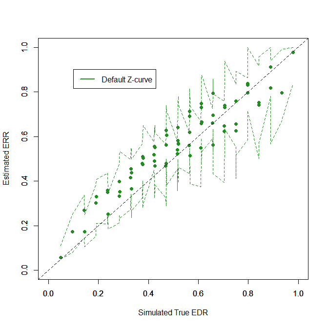
Figure 5 shows the fit for both methods (default z-curve = green, NDIST zcurve = purple). The figure shows that both methods do reasonably well, but the default method performs better. The following statistical tests compare the fit of the two models quantitatively.

The RMSE is the square root of the mean squared differences of the true and estimated ERRs. The values are .008 for the default method and .029 for the NDIST method. The directional bias of the default method ranged from -2.5 percentage points to 2.6 percentage points. The directional bias for the NDIST method ranges from -5.0 percentage points to 7.4 percentage points. All of the z-curve confidence intervals included the true value, but only 58% of the confidence intervals for the NDIST method included the true value. This could be fixed by crating conservative confidence intervals to ensure good coverage for the NDIST method, but what would be the point. The default method works better. The NDIST method is not bad – and better than p-curve (Chapter 5), but it makes an unnecessary assumption that lowers performance.

Expected Discovery Rate

The results for the expected discovery rate are presented in two different figures because a combined plot was too messy. The results for the default z-curve show that estimating the EDR from only significant results is difficult. The estimates are not tightly clustered around the diagonal. However, the confidence intervals are on both sides of the diagonal, showing that most of them include the true value.

Results look different for the NDIST method. Performance was bad, to use scientific language.

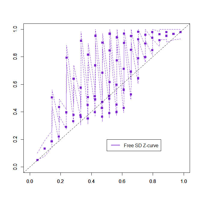
The example shows why. The assumption of a normal distribution often underestimates the amount of non-significant results. A formal comparison is hardly necessary, but here are the results. The RMSE is .088 for the default method and .218 for the NDIST method. Directional bias ranged from -14 to 16 percentage points for the default method and from -18 to 58 (!!!) percentage points for the NDIST method. Coverage of confidence intervals was 89% for the default method and 26% for the NDIST method. Coverage should be 95% for the default method, but the EM method may do better. Coverage of confidence intervals with the EM method will be examined in another chapter.

Conclusion

Simulations are used to evaluate the performance of statistical methods. The advantage of simulations is that we know the “simulated” truth. Simulations that match all of the assumptions of a model are not very useful because they will show that a method does well. It is more interesting to examine how a model performs when assumptions are not, especially when these assumptions cannot be tested in real data. In the present simulation, we knew that the simulated distribution of non-central z-values was not normal and tested how well a model that assumes a normal distribution performs. The results showed acceptable performance for estimates of the ERR, but unacceptable performance for estimates of the EDR.

The advantage of the default method is that it does not make assumptions about the unknown distribution of the non-central z-values. This is why it is the default method. Although the method is not as good when the distribution of the non-central z-values is normal, the method approximates the true distribution reasonably well. The reverse is not true.

The results have broader implications for effect size meta-analyses. The best method to correct for bias and allow for heterogeneity in effect sizes is the random effects selection model implemented in the R-package weightr. The key drawback of the method is that it assumes a normal distribution of population effect sizes. This is not a realistic assumption, but it has not been evaluated how robust the method is when the assumption is violated. Finally, it may be worthwhile to develop methods that do not require assumptions about the distribution of effect sizes (a z-curve for effect sizes).