In this blog post, I continue and expand my exploration of Carter et al.’s (2019) extensive simulation studies of meta-analytic methods. I focus on Carter et al. because it was a seminal study and remains the most thorough study so far. It also remains the key article that is being cited in applied articles to interpret conflicting results.
My previous posts reproduced Carter et al.’s (2019) simulations exactly. In my “Beyond Carter” series, I am starting to investigate new scenarios that were not considered in their design. This is the first blog post in this series. It focuses on the influence of sample sizes in the original studies on the performance of various methods. Carter et al.’s (2019) used a distribution of sample sizes that included many studies with large samples. This is not immediately obvious because their figure was truncated at N = 400.
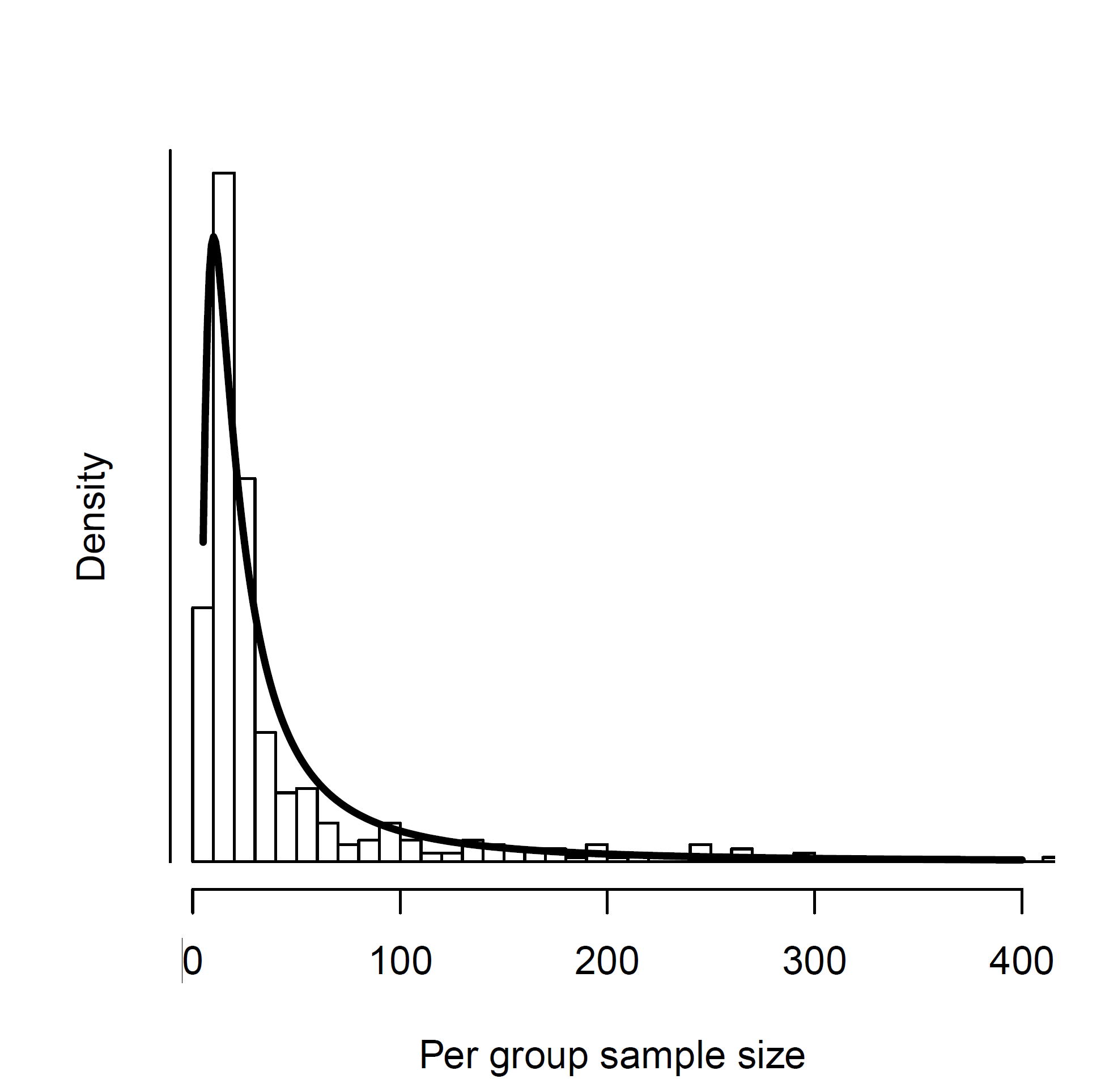
However, the actual sample sizes were not truncated at N = 400, although studies with more than 800 participants are rare in experimental psychology, even in the days of online studies. The use of a single distribution of sample sizes is problematic because results based on these simulations may not generalize to meta-analysis with smaller sample sizes. It is also problematic to make recommendations about the interpretation of conflicting results based on these simulations. A more sensible approach would be to ask researchers to perform a simulation study with the sample sizes that match the sample sizes of their actual dataset. After all, sample sizes are known knowns, and not untestable assumptions.
In this blog post, I used the sample sizes of Carter et al.’s (2019) ego-depletion meta-analysis to see how robust their recommendations are to changes in sample sizes. To keep all other aspects of the simulation the same, I used Carter et al.’s simulation function and created more studies than needed. I then sampled from this set of studies to match the percentage of studies with very small (39% N < 40; ), small (52%, N = 40 – 100), medium (8% N = 100 – 200), and large (1% N = 200-400) studies in the ego-depletion dataset.
The first blog post uses Carter et al.’s Simulation #328 with k = 100 studies, an average population effect size of d = .2, a standard deviation of normally distributed population effect sizes (tau) of .4, no selection bias, and high amount of p-hacking. The results for the simulation with Carter et al.’s sample sizes showed that p-hacking introduces a small (d = .1 to .2) downward bias in the effect size estimates for all methods (). The question is whether smaller sample sizes increase that downward bias and whether some methods are more affected by p-hacking when sample sizes are small.
Random Effects Meta-Analysis
I added the standard random effects meta-analysis model to my simulation studies. The main reason is that the results serve as a benchmark to evaluate bias-correction methods. If bias is small, the benefits of correcting for bias may out-weight the costs of doing so. Carter et al.’s (2019) study already showed that p-hacking and selection bias have different effects on random effect meta-analysis. Namely, p-hacking – as simulated by Carter et al. (2019) – introduced only a small bias in effect size estimates.
This observation was confirmed here. The average effect size estimate was d = .38, average 95%CI = .28 to .49, and 70% of the confidence intervals included the true value of d = .30. The model also slightly overestimated the true heterogeneity, average tau = .46, 95%CI = .35 to .54. While there is some bias in the estimates, they do not radically change the conclusions. Moreover, it is not clear that bias-correction models can do better in this scenario.
It is also instructive to compare this result with Carter et al.’s (2019) ego-depletion RMA result that produced an effect size estimate of d = .43, 95%CI = .34 to .52. Carter et al. (2019) dismiss this finding because the model has a high false positive risk when the null hypothesis is true, but this does not mean that it would produce estimates of d = .4 when the null hypothesis is true. The present simulation suggests that the result could be obtained with a small average effect size, high heterogeneity, and p-hacking.
Selection Model
An improved selection model that accounts for p-hacking did well in the simulations with Carter et al.’s (2019) sample sizes, but it struggled in this simulation with smaller sample sizes. It often failed to estimate all of the parameters, and the effect size estimate failed to reject the false null-hypothesis.
The advantage of the selection model is that it can be modified, if it fails to work well. One problem for the selection model was that Carter et al.’s (2019) simulation contained several negative values, including some statistically significant ones. To reduce the number of steps, it is possible to remove all negative values and to specify this selection with a step at p = .5 (one-sided). The model will then use a fixed value of .01 and does not need to estimate this weight parameter, making it easier to estimate free parameters.
However, even this modification was not sufficient to identify all parameters reliably. The problem was that there were not enough just-significant p-values to estimate the parameter for p-hacked p-values between .005 and .025. A solution to this problem was to widen the interval to .005 to .05. This is even more reasonable with real data because p-hacking also often leads to marginally significant results (.025 to .05) that are presented as evidence against the null-hypothesis. A model with a single parameter for just significant (.005 to .025) and marginally significant results (.025 to .050) can be used when the set of studies is relatively small. The modified selection models with steps = c(.005, .050, .500, 1) produced estimates in 99% of the simulations.
The true average effect size was d = .30. The true average is higher than d = .20 because the selection of different sample sizes changed the population of studies, and the new population had a higher average. The average effect size estimate was d = .32, average 95%CI = .31, 95%CI = .22 to .43, and 67% of confidence intervals included the true average. Thus, the model showed a small upward bias, but it was able to do a bit better than the random effects model that ignored bias.
To compare the performance of the selection model to models that focus on positive results or positive and significant results, I used the estimated average and standard deviation of population effect sizes to estimate the average effect size for these populations of studies. The true average for only positive results was d = .38. The average selection model estimate was d = .46, average 95%CI = .21 to .65, and 65% of confidence intervals included the true value. Thus, upward bias is also present for this subset of studies.
The true average for positive and significant results is d = .50. The average estimate was d = .65, average 95%CI = .25 to .88, and 94% of confidence intervals included the true average. The bias is larger, but the wider confidence intervals produce better coverage than the estimates for other sets of data.
The point estimate of heterogeneity was good, average tau = .39 (true tau = .4), but the average 95% confidence intervals was wide, .04 to .57. The wide confidence intervals included the true value 91% of the time.
The model correctly identified selection of significant results in all simulations. The highest estimate of the selection weight for non-significant positive results was w = .65, and the highest upper limit of the confidence intervals was w = .89. Thus, the model can be used to detect selection bias and warn against the use of models that do not take biases into account.
The model noticed p-hacking. That is, the average selection weight for just significant results was well above 1, average w = 2.32, but the average 95%CI was wide, 0.64 to 3.84, and only 13% of confidence intervals rejected the null hypothesis of no p-hacking. Thus, it is difficult to diagnose p-hacking in this simulated condition.
Overall, the performance of the selection model was negatively affected by smaller sample sizes in the original studies (not a smaller set of studies). The full model that produced good estimates before had identification problems. A modified model failed to fully correct for p-hacking, and the confidence intervals often did not include the true value. While the results were not terrible, there is room for other models to do better. At the same time, the model correctly identified heterogeneity and selection bias. Thus, the model should always be used to examine assumptions. A fixed effect size model without bias should not be based after the selection model shows evidence of heterogeneity and bias.
PET-PEESE
The PET-PEESE model was strongly influenced by the change in sample sizes. PET regresses effect size estimates on sampling error. With fewer studies that have large samples and small standard errors, the prediction of the intercept becomes more uncertain as reflected in larger sample sizes. Moreover, absent unbiased estimates close to the intercept, the correction for p-hacking is more difficult. This led to a strong downward bias in effect size estimates, average d = -.57, average 95%CI = -1.84 to .71. Although 74% of the very wide confidence intervals included the true value of d = .27, none of the confidence intervals rejected the false null hypothesis.
It is instructive to compare these results to the PET results for the actual ego-depletion meta-analysis, d = -.27, 95%CI = -.52 to d = .00. The results also show a negative estimate and fail to reject the null hypothesis. Although the confidence interval is narrower, the pattern qualitatively matches the original results. Thus, p-hacking and small samples may have produced the negative estimate in the actual meta-analysis. This would undermine Carter et al.’s conclusion that PET is most likely to produce the correct results based on their simulations with larger sample sizes.
PEESE is a regression of effect size estimates on the sampling variance (i.e., squared standard errors). PEESE estimates are only used if PET produces a positive and significant result. Thus, they are irrelevant in this simulation, but even PEESE produced negative estimates, average d = -.14, average 95%CI = -.19 to -.09. The confidence intervals are narrower. These results are even more similar to the results for the actual ego-depletion data, d = .00, 95%CI = -.14 to .15.
In conclusion, the combination of small sample sizes and p-hacking leads to a strong downward bias for PET estimates. This also influences the overall result of PET-PEESE because non-significant or negative PET results are given priority in effect size estimation to avoid overestimation with PEESE. However, if PET has a strong downward bias, PEESE results are actually better, questioning the priority of PET in the interpretation of results.
I also added an additional analysis of the data to explore the reason for the downward bias in PET-regression. For this purpose, I examined the correlation between sampling error and the POPULATION effect sizes. Without bias, the simulation assumes that the two are not correlated. That is sample sizes are randomly paired with population effect sizes. However, p-hacking produces a correlation between sampling error and population effect sizes, average r = .39. PET assumes that this correlation is zero and that any correlation between sampling error and the effect size estimates reflect bias. This will lead to a downward bias in the estimates when the assumption is false and studies with smaller sampling error have smaller effect sizes. This bias will vary as a function of the estimated correlation in a specific simulation. This is indeed the case. The bias in PET estimates was negatively correlated with the correlation between sampling error and population effect sizes, r = -.42. Future work needs to explore how p-hacking creates a correlation between sample sizes and the true population effect sizes. For now, these results explain why PET regression has a downward bias. This problem has been overlooked in previous tests of PET regression because simulations either did not simulate p-hacking (Stanley, 2017) or the dataset included many studies with large samples that minimize downward bias (Carter et al., 2019).
The key finding is that negative PET estimates suggest that PET estimates have a downward bias and that PET-PEESE should not be used, when better alternatives are available. It is especially problematic to use negative PET results as evidence that the average effect size is zero, when other models produce positive effect sizes (Carter et al., 2019).
The poor performance of PET-PEESE in this simulation is not unexpected. The parent of PET-PEESE pointed out that PET-PEESE can be unreliable when bias is present and (a) there is little variability in sample sizes of original studies, (b) the sample sizes are small and observed datapoints are far from the intercept. The present analysis only adds that p-hacking makes things worse and produces a strong downward bias and negative estimates when the average effect size is small. The only reason to use PET-PEESE would be that it performs better in other conditions, but so far the selection model always performed as well or better than PET-PEESE. Thus, there is no reason to use PET-PEESE, especially because it is difficult to detect p-hacking. Maybe the main reason to use PET-regression is to use negative estimates as a test of p-hacking.
P-Uniform
P-uniform uses only positive and significant results and estimates the average effect size of this set of results. Carter et al. (2019) claimed that p-uniform overestimates effect sizes, but this claim was based on the false assumption that p-curve estimates the effect size for all studies. This is only possible if all studies have the same population effect sizes and all subsets of studies have the same effect size (i.e., tau = 0). I found that p-hacking actually also produces a downward bias in p-uniform estimates as it does for all models that assume bias was produced by selection bias when it was actually produced by p-hacking.
P-uniform also has a bias test, but only 5% of bias tests were significant, which is expected by chance alone. Thus, the selection model should be used to test for the presence of bias.
P-uniform underestimated the average effect size of studies with positive and significant results, average d = .33, average 95%CI = .05 to .53, and 64% of confidence intervals included the true value of d = .50. The performance is about the same as the selection model, but with opposite biases.
Carter et al.’s (2019) ego-depletion results showed an estimate of d = .55, 95%CI = .33 to .71. The present results suggest that this finding is consistent with a scenario with a small average effect size, high heterogeneity, and p-hacking. The higher estimate in the actual data may be due to less severe p-hacking than in this simulation.
P-Curve
Carter et al. (2019) used p-curve to estimate effect sizes. I did not include p-curve for this purpose in my previous posts because the results are similar to p-uniform and p-uniform has an R-package. Here I am included p-curve estimates of power. The reason is that p-curve is much more often used to examine evidential value and bias than to estimate effect sizes. Often p-curve is used in combination with traditional meta-analysis to claim that estimates without bias correction are acceptable because p-curve showed evidential value.
The inclusion of p-curve is also interesting to compare its performance with z-curve, another method that focuses on power rather than effect sizes. Z-curve has the advantage that it models heterogeneity in power and produces better estimates when heterogeneity is high (Brunner & Schimmack, 2020). The p-curve authors have claimed that the superior performance of z-curve occurs only in rare cases with extreme outliers (Datacolada, 2018). Thus, it is interesting to test this claim with standard meta-analytic scenarios.
P-curve estimates the average power of positive and significant results. The average estimate was 32%, average 95%CI = 18% to 47%, and 70% of the confidence intervals included the true value of 38%. The results shows again a downward bias because p-curve corrects for inflation assuming selection for significance, but p-hacking introduces a smaller bias. This leads to an underestimation of the true value. However, the bias is relatively small.
P-curve sometimes uses the arbitrary criterion of 33% power to examine whether a set of significant values has acceptable average power. Only 14% of simulations rejected the hypothesis that power is at least 33%. This finding is not very interesting when the true power is 38%. There is no meaningful difference between 28% and 38% power.
The most interesting result is that p-curve produced a relatively good estimate of average power despite high heterogeneity in effect sizes. The reasons for this good performance become clearer in the analysis of the data with z-curve.
Z-Curve
One advantage of z-curve is that a z-curve plot provides some information about bias. To illustrate this, I am presenting the results of a z-curve plot with k = 5,000 studies. The actual results are based on the same simulation data as for the other models.

Figure 1 shows a plot of the 735 results with a positive z-value (z-values are obtained by transforming the t-values obtained from effect size estimates and sampling error into z-values). Visual inspection of the pattern shows missing non-significant values and too many just significant results. Just significance is arbitrarily defined by p-values between .05 and .01, which corresponds to z-scores between 2 and 2.6. The test of excessive just significant results is highly significant with k = 735 tests. The pattern suggests that the excess of just significant results was obtained by p-hacking some of the non-significant results. However, other ways produce this pattern of results are possible. This makes it difficult to correct for p-hacking.
In the simulation, I tried to test for p-hacking by fitting the z-curve model to the “really” significant results (z > 2.6) and seeing whether there are too many just significant results. However, this test has low power and cannot be performed when there are only few “really” significant results, p < .01. With k = 100, the test did not work. Thus, I fitted the normal selection model that assumes excessive just significant results are due to not publishing results non-significant results.

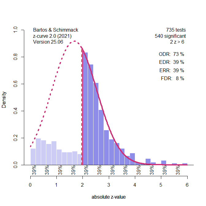
Figure 2 shows the result. The expected replication (ERR) is a different name for the average power of the positive and significant results and can be compared with the p-curve estimate. In this single simulation, the estimates are similar, 29% versus 32%, but the real comparison has to use the same data. The main point here is that p-curve does better than z-curve in this scenario. The reason is that p-curve results have two biases. Estimates have a downward bias when selection is assumed, but p-hacking was used. This is true for all models. In addition, p-curve has an upward bias when the data are heterogeneous. When p-hacking and heterogeneity are present the two biases cancel each other out. However, in real data it is not known how much p-hacking was used and the upward bias may lead to inflated estimates. This bias can be severe. It is therefore problematic to rely on p-curve estimates alone. In combination with z-curve and a plot like the one in Figure 1, p-curve results may be interpreted as a better correction for p-hacking. An alternative approach is to use z-curve estimates and use the biased estimates as conservative estimates rather than to correct estimates upward. This would be a p-hacking penalty. Given the uncertainty about the practices that were used to p-hack data, this might be considered an appropriate correction.
One advantage of z-curve over p-curve is that it provides tests of bias. The test of excessive just significant results produced on average 60% just significant results when the model only predicted 40%, and 96% of the significance test were significant. The performance of the selection model was better, but it sometimes fails to provide estimates. Using both tests should produce convergent evidence that bias is present.
The average estimate of average power for positive and significant results (average ERR) was 28%, average 95%CI = 12% to 47%, and 81% of the confidence intervals included the true value. It is noteworthy that the coverage of the confidence interval is better than the coverage of p-curve confidence intervals, although the downward bias was more pronounced. This shows that p-curve confidence intervals are too narrow, which has been observed before (Shane et al., 2019). However, p-curve estimates were on average less biased than z-curve estimates (average bias -6 vs -10 percentage points). This difference is not practically significant, and both methods lead to the same conclusion in this simulation.
Z-curve extrapolates from the distribution of significant results to estimate the average power of all positive results, significant and non-significant ones. P-curve does not do this because it assumes homogeneity. If all studies have the same power, power is the same before and after selection for significance (Brunner & Schimmack, 2020). Thus, we can also use the p-curve estimate of 32% as an estimate of the average power for all positive results.
In this specific simulation, p-curve is lucky and hits the nail on the head. The estimate of 32% matches the true value exactly. In contrast, z-curve produces a lower estimate of 15%, 95%CI = .05 to 36%. Thus, the downward bias introduced by p-hacking has more severe effects on this estimate. Better ways to detect and correct for p-hacking are therefore needed to keep the p-hacking penalty at a reasonable level.
One approach is to create a p-curve version of z-curve. This means, the model uses only a single parameter to fit the data. In addition, the model allows the standard deviation of the normal distribution to be freely estimated rather than assuming a fixed value of 1. In this model, the peak of the normal distribution was estimated to be 1.68 (see Figure 3) and the standard deviation was less than 1, SD = .86.
The SD below 1 is the result of p-hacking that leads to a bunching of z-values in the just-significant range. The model cannot fit the distribution of the really significant results, but there are very few. As a result, this model provides an even better estimate of average power than p-curve, ERR = 39%, true value = 38%. This may just be a lucky result, but allowing for a free component with a free mean and free SD may be a way to capture p-hacking with z-curve.
A new extension of z-curve is to convert power estimates into effect size estimates. The simplifying assumption to make this possible is to assume that population effect sizes are independent of sample sizes. Assuming positive or negative correlations would produce different estimates. In the present simulation, it was already shown that the independence assumption is false and biased PET regression results.
The average effect size estimate for positive and significant results based on z-curve estimates of power, however, were only slightly biased, estimated average d = .44 , average 95%CI .22 to .60, and 90% of confidence intervals included the true value of d = .50. However, the confidence intervals were wide and only 61% of confidence intervals did not include a value of d = .2, the value for a small effect size. This performance is better than the performance of p-uniform and the selection model.
The average estimate for the effect size of all positive results based on the power estimate for this set of studies was d = .28, average 95%CI = .02 to .51, and 76% of confidential intervals included the true value of d = .42. Only 5% of confidence intervals did not include a value of .2. Thus, the downward bias made it difficult to show that the effect size is not small. The selection model performed better.
Conclusion
The main finding in this simulation was that all models except PET-PEESE provided positive estimates of the average effect size for all studies or subsets of studies. P-curve and z-curve also showed that the studies with positive and significant results are not all false positive results. That is, the null hypothesis is clearly rejected at least for a subset of studies.
Why is this important? This finding is important because it mirrors Carter et al.’s (2019) results for actual studies of ego-depletion (see Figure 4, a copy of their Table 2).
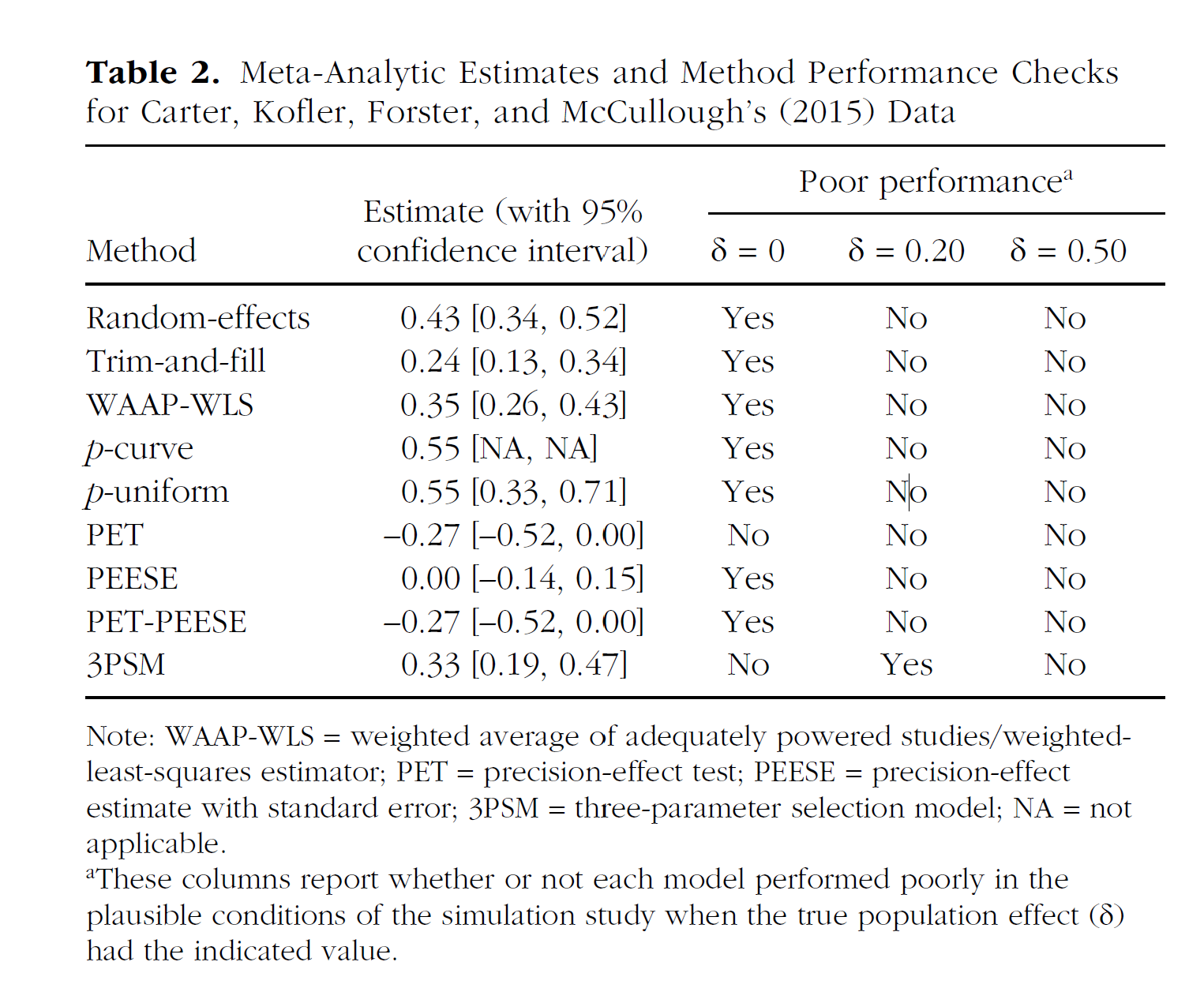
However, Carter et al. (2019) used their simulation studies to suggest that PET-PEESE results are the most trustworthy results because PET-PEESE showed the best performance in simulations without a real effect. Thus, the finding that PET-PEESE did not show a positive effect, while the other models showed one, was interpreted as evidence that the average effect size is probably zero, and implicitly as evidence that estimates of the other models are false rejections of a true null hypothesis.
The present results undermine this conclusion with a simulation that is identical to their simulations of p-hacking, but with sample sizes that match the ego-depletion literature. As the present simulation uses sample sizes of the actual ego-depletion studies, the results are more relevant than simulation results with other sample sizes that make PET-PEESE perform better. It is therefore necessary to revise Carter et al.’s (2019) conclusions about PET-PEESE and the interpretation of the ego-depletion meta-analysis. First, it is extremely unlikely that all significant results in the ego-depletion meta-analysis were false positive results. This does not mean that it is easy to replicate any particular study because hidden moderators may make it difficult to replicate these studies, but it does mean that ego-depletion manipulations sometimes had at least a small effect on some dependent variable. More importantly, the results mean that PET-PEESE is not as robust as Carter et al.’s (2019) table and online app suggests. The table suggests that PET-PEESE performs well with small effect sizes. I showed that this is not the case and that downward bias can turn a small positive average effect size into an estimated moderate negative effect. The difference between the true and estimated values is large (d > .5). Thus, it may be necessary to reexamine meta-analysis that relied on PET-PEESE to suggest that a set of studies lacks evidential value.
The results also imply that it is necessary to revisit other scenarios in Carter et al.’s simulation study with other compositions of sample sizes, especially sets of studies with small to medium sample sizes that lack large sample sizes that produce unbiased estimates. In other words, Carter et al.’s (2019) article was a good start, but not the final word on the performance of meta-analytic methods under realistic conditions.