In a nutshell

Statistical methods for meta-analyses make different assumptions. For this reason, different methods can produce different results with the same data. Meta-analysts often struggle to make sense of these inconsistent results. A simple solution to this problem is to test testable assumptions. Key assumptions that influence results are publication bias and heterogeneity of population effect sizes. Here I show how testing these assumptions explains inconsistencies in results and that methods that violate assumptions produce biased results. I also show with two examples (ego-depletion, terror management) and tailored simulation studies that different methods produce similar results when the same data are used. Differences in results in the terror management multiverse meta-analysis were found to be due to the analysis of different datasets. The article clarifies many misconceptions about multiverse meta-analysis and helps applied researchers and readers to make sense of these studies.

Introduction

Meta-analysis is nearly as old as inferential statistics itself. Genius and eugenicist Sir Fisher developed the first meta-analysis using p-values rather than effect sizes. He also developed the first bias test for meta-analysis and showed that Mendal’s famous data of dominant and recessive genes in peas were too good to be statistically true. In this case, of course, the main finding remained true.

Effect size meta-analysis emerged in the 1960s to make sense of conflicting results in original studies with small sample sizes that lacked statistical power to detect small to moderate effects in a single study (Cohen, 1962).

When we can assume that the available data are an unbiased sample and all studies estimate the same population effect size, it is rather simple to meta-analyze the data. A simple average of effect sizes will do. A better solution is to weigh the data by sample size or similar weights (inverse of sampling error, inverse of sampling variance). Voila, you have the best estimate of the population effect size.

In reality, meta-analytic results can produce dramatically false results for two reasons. First, effect sizes may vary across studies due to a number of factors. For example, effects (or statistical relationships in correlational studies) can vary across populations. Variability in effect sizes is called heterogeneity. Hundreds of articles have discussed the problem of heterogeneity and how to deal with it in meta-analyses.

The second problem is that existing studies may be biased towards evidence for an effect. For example, a meta-analysis of extrasensory perception suggested that it is real. This is known as publication bias. Standard meta-analysis will overestimate effect sizes when publication bias is present. For example, the Open Science Collaboration Reproducibility Project (2015) showed that a naive meta-analysis of psychological studies would overestimate effect sizes by 100%. If a meta-analysis of diets suggests that the average weight loss is 50ls, the real effect is only 25lb. Even more dramatic examples can be found. A naive meta-analysis of ego-depletion (loss of willpower) suggested an effect of .6 standard deviations. A bias-corrected meta-analysis and credible replication studies suggest that the effect may not exist or is very small (< .1 standard deviations); an inflation by 600%.

During the credibility revolution, interest in statistical methods that can detect and correct for publication bias has increased tremendously. To ensure robustness of results, it is often recommended to use multiple methods (Carter et al., 2019). The use of multiple methods to test robustness has become known as a multiverse analysis. Unfortunately, multiverse meta-analyses often produce inconsistent results. As a result, meta-analytic articles often produce no clear conclusions (Cheng et al., 2025).

In this article, I argue that lack of robustness is to be expected because different meta-analytic models make different assumptions. Although it is widely acknowledged that valid statistical inferences require valid assumptions, testing of assumptions is often ignored (Nimon, 2012). This is also true for multiverse meta-analyses. Even when methods test assumptions, the results of this tests are often ignored (Carter et al., 2010; Cheng et al., 2025). In this article, I illustrate with simulations and two actual datasets how testing of assumptions resolves seemingly inconsistent effect size estimates. Some of these inconsistent results are based on false assumptions and are invalid because sound inferences require valid assumptions.

However, untested assumptions are not the only reason for inconsistent results. I show two additional problems in multiverse meta-analyses. First, sometimes models are mis-specified when default assumptions do not fit a dataset (Cheng et al., 2025). Second, sometimes the input data for different methods differ substantially and lead to different conclusions (Cheng et al., 2025).

I use the results from Carter et al.’s (2019) multiverse meta-analysis for educational purposes. The data are from a real dataset with 116 ego-depletion studies. The results in their Table 2 showed that different methods produced different average effect size estimates that “would lead to different conclusions” (p. 139). As can be seen in the table, the average effect size estimates range from -.27 standardized mean differences (SMD), a small negative effect, to an SDM of .55, a strong effect. Subsequently, I show that this large range of estimates is not as inconsistent as it seems to be. Rather, the results are all consistent with (a) the presence of publication bias, (b) the presence of heterogeneity, and (c) a moderate to strong effect for positive results that were statistically significant.

Test for Publication Bias

Some methods used by Carter et al. (2019) provide information about publication bias, but this information was not used by Carter et al. to interpret the results in Table 2 Specifically, PET and PEESE use regression of effect sizes on sampling error to examine publication bias. Publication bias produces a positive correlation between sampling error and effect sizes because significance requires larger effect sizes in studies with larger sampling error. PET showed a strong correlation in the ego-depletion data. Based on this finding, we could reject results of methods that do not correct for publication bias and conclude that the true effect size is close to zero (negative values seem implausible). However, 3PSM also tests and corrects for publication bias and produces a positive estimate of SMD = .33. P-curve and p-uniform do not test for bias, but correct for it when it is present. They also produce positive estimates.

However, the results of PET/PEESE and p-curve and p-uniform are not as inconsistent as they may appear. The reason is that these methods estimate the average effect size for different sets of studies. PET/PEESE estimates the average effect size for all studies, whereas p-curve and p-uniform estimate the average effect size for studies with significant results. As larger effect sizes are more likely to produce significant results, these methods select for larger effect sizes, if there is heterogeneity in effect sizes. Thus, inconsistency may be simply a function of heterogeneity in effect sizes. It is therefore important to test this assumption as well.

Test for Heterogeneity

In the presence of publication bias, the traditional random effect-size meta-analysis cannot be used to test heterogeneity in effect sizes because publication bias is likely to produce heterogeneity when sample sizes vary. The only method used by Carter et al. (2019) that takes publication bias into account and tests heterogeneity is the 3PSM model. I first reproduced Carter et al.’s (2019) results with the default specifications that assumes selection for statistical significance at p = .05 (two-tailed), average effect size estimate, g = ..33, tau = .38. However, these default settings make some untested assumptions. For example, they assume that positive and negative non-significant results are equally likely to be reported. This can be tested by adding a step at p = .5 (one-sided). This did not change the results. The model also assumes that marginally significant results (.10 < p < .05, two-tailed) are as likely to be reported as other non-significant results. This can be tested by adding a step at p = .05 (one-tailed). This modification also did not change the results. Another possibility is that p-hacking produces many just significant results. This assumption can be tested by adding a step at .005 (one-sided). This led to an even higher estimate of the average effect size, g = .46. In short, the estimate with the default model is robust to various alternative specifications that make different assumptions about selection bias. The results show evidence of large heterogeneity in effect sizes.

It is not possible to compare this average effect size estimate directly with p-curve and p-uniform because the latter methods focus only on significant positive results. To make the 3PSM results comparable, it is possible to estimate the average for only significant results using the predicted density distribution of effect sizes from the 3PSM model.

The average for only positive effects is g = .53. This is close to the estimates for p-curve and p-uniform, g = .55 and does not take into account that selection for significance would further increase the average effect size. A simulation that assumes no correlation between effect size and sampling error produced an estimate of g = .67, which is even higher than the estimate obtained with p-curve and p-uniform.

In conclusion, there is evidence of publication bias and heterogeneity in effect sizes and strong average effect size for studies with positive population effect sizes. This result is consistent with p-curve and p-uniform estimates that positive significant results were obtained with a large average population effect size.

The key inconsistency is between the PET/PEESE estimate of a negative average effect size, but even this inconsistency is more apparent than real. First, the average for all studies can be consistent with a large positive average for a subset of studies when heterogeneity is present. Second, PET/PEESE does not perform well when large heterogeneity is present and few studies produce precise estimates of the population effect size in large samples. Another problem is that this model relies on the correlation between effect sizes and sample sizes to correct for bias. When other factors produce a correlation, the model will overcorrect and underestimate the average effect size estimate. The 3PSM model does not have the same problems and performs well in simulations with high heterogeneity (McShane et al., 2016).

The New Kid on the Block: Z-curve 3.0

Z-curve was still under development when Carter et al. (2019) published their article. Since then, z-curve has been validated and extended (Brunner & Schimmack, 2020; Bartos & Schimmack, 2022). The main aim of z0curve is not to estimate average effect sizes and it is not commonly used in multiverse meta-analyses. However, z-curve can provide valuable information about publication bias that can supplement the results of the 3PSM model. It also provides information about heterogeneity. A new extension of z-curve adds two direct tests of heterogeneity, one without assumptions about the distribution of population z-scores (i.e., the expected value in a large number of exact replication studies), and one assuming a normal distribution that also estimates the amount of heterogeneity. Another extension of z-curve transforms the z-curve estimates of power into effect size estimates to make the results more comparable to the results of effect size models. To do so, power is used to compute the corresponding non-central t-value based on the degrees of a study. The non-central t-values are then converted into effect size estimates, and the weighted average of these estimates is the estimate of the average effect size. Z-curve produces estimates for two populations of studies. One estimate can be compared to p-curve and p-uniform estimates that focus only on significant results. The other one can be compared to the 3PSM model and focuses on all positive results.

To use z-curve, effect sizes and sampling error are used to compute t-values, and the t-values are converted to z-scores. For this analysis, negative z-scores were excluded, leaving k = 92 z-scores for the analysis.

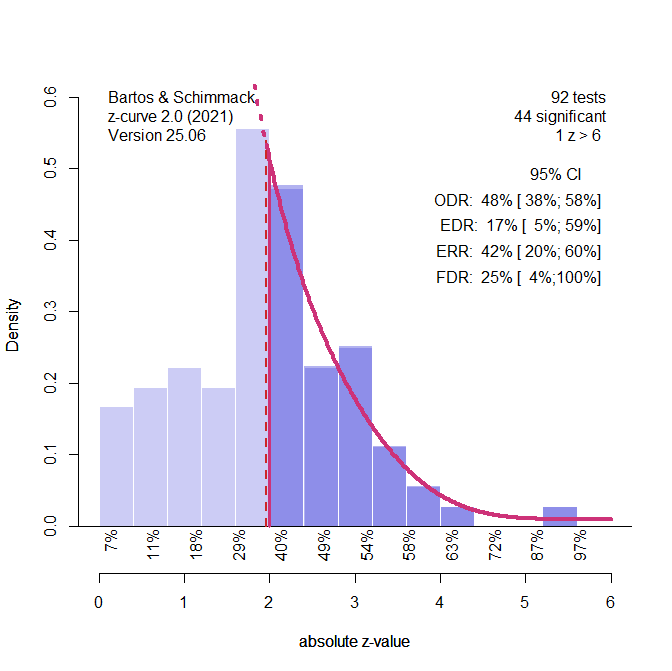
Visual inspection of the histogram shows an abnormally high number of results close to the level of significance for two-sided z-tests, z = 1.96. This concentration of results close to p = .05 is a sign of publication bias or p-hacking (i.e., the use of statistical tricks to get a p-value close to .05). The standard z-curve model assumes publication bias rather than p-hacking. This implies that for every weak significant result there are many non-significant results from studies with equally low power. This assumption is reflected in the low estimated of the Expected Discovery Rate (17%) that implies that 100 attempts produced only 17 significant results. However, due to the small set of studies, there is a lot of uncertainty in this estimate, 95%CI = 5% to 59%.

The expected replication rate is an estimate of the power of the subset of studies with significant results to produce a significant result again in an exact replication study with the same sample size. The average power for this subset of studies is 42%. The difference between the EDR and ERR implies heterogeneity. If all studies had the same power, selection for significance could not select a subset of studies with higher power.

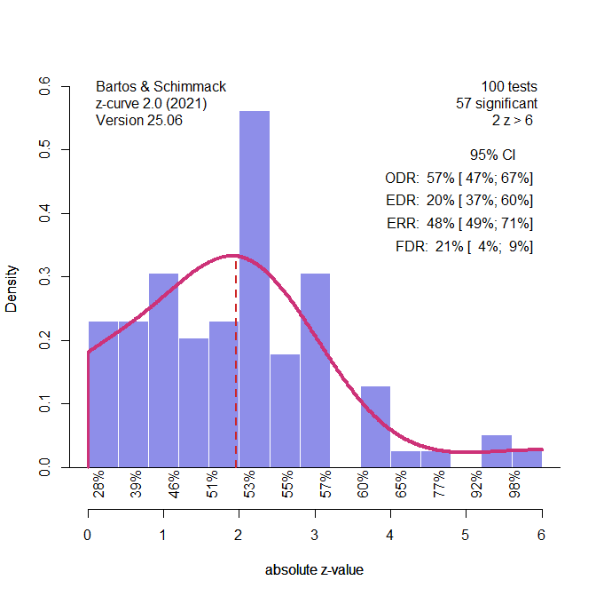
Figure 2 shows an alternative specification of z-curve. This model assumes that there is no publication bias and non-significant results are included in the analysis. The results show that the predicted z-score distribution fits the observed on pretty well, except for the results around p = .05. This could be explained with p-hacking rather than selection for significance. The main effect on the results is an increase in the EDR from 17% to 49%. Thus, there is some uncertainty about the average power of studies before selection for significance because this estimate depends on assumptions about the cause of bias in the data: publication bias or p-hacking, but both estimates agree that statistically significant results have modest average power around 40% to 50%.

Heterogeneity Test 1

A new extension of z-curve makes it possible to test heterogeneity further. The first test compares a one-component model (all studies have the same power) with a two component model (there are two populations of studies with different levels of power (say 20% and 80%). A bootstrap method is used to compute 500 difference scores of model fit and use CI to compare the results against a value of zero. Difference scores are computed so that higher values imply better fit (homogenous – heterogenous model fit). The value for the one-sided 90% CI was 0.00, indicating no better fit for the heterogenous model. A power test that increased the same size 20-fold still showed no significant evidence of heterogeneity in power.

Heterogeneity Test 2

A second test assumes that power varies only slightly and that is variation is normally distributed. This model is similar to the 3PSM model except that it makes an assumption about the distribution of power rather than effect sizes. To model this assumption, the one component model with a fixed SD of 1 is compared to a one-component model with a variable SD. Even this model showed no evidence of heterogeneity, fit difference, 90%CI = 0.00. The 95%CI for the SD parameter ranged from 1 to 1.35. The problem for z-curve is that the data are consistent with a model with fixed moderate power (M = 1.74, SD = 1) or a model with low average power and modest heterogeneity (M = 1, SD = 1.29).

This result seems inconsistent with the estimate of higher heterogeneity in effect sizes with the 3PSM model, but there is a possible explanation. If POPULATION effect sizes are correlated sampling error, the heterogeneity in effect sizes does not produce heterogeneity in power because larger effect sizes are tested with more sampling error. This would also explain why PET/PEESE underestimates the average effect size compared to other models. A true correlation between effect sizes and sampling error is falsely assumed to be caused by publication bias and the model overcorrects for the bias that is not present.

In this regard, a comparison of heterogeneity in effect sizes with 3PMS and power with z-curve can be used to diagnose to test the assumption of PET/PEESE that population effect sizes are unrelated to sampling error.

Effect Size Estimation with Z-Curve

Z-curve can also be used to estimate effect sizes. A simple way of doing so, is to convert the average power into t-values based on the degrees of freedom of a study and then to convert the t-values into d-values and compute the average effect size. Using the ERR estimates that assume selection for significance produces estimates that can be compared to the p-curve and p-uniform estimates. The z-curve estimate based on the ERR is d = .57, 95%CI = .31 to .67, which is in line with the other methods. The EDR can be used to estimate the effect size for positive results without selection for significance. The estimate is lower than the 3PSM estimate, d = .35, but the 95%CI is wide and ranges from d = 00 to .67. This range includes the 3PSM results.

Conclusion

Carter et al. (2019) suggested that results of multiverse analyses are difficult to interpret because of the “dependence of meta-analytic methods on untestable assumption” (p. 116). Rather than advocating for the test of underlying assumptions, they suggested that researchers should draw conclusions based on plausibility judgments about the presence of bias or heterogeneity. Based on this logic, they rely on simulation studies to argue that the PET-PEESE results are most likely to reveal the true average population effect size because “the PET
method does not perform poorly in any of the plausible conditions we examined” (p. 139).

The present results cast doubt on the validity of this inference that was based on simulated data rather than the data under investigation. Moreover, Carter et al. (2019) ignore the evidence of heterogeneity in effect size estimates. When heterogeneity is present, PET-PEESE only estimates the mean effect size of all studies with positive and negative population effect sizes. Even a negative mean can be consistent with the finding of other methods that the average effect size for studies with positive population effect sizes is substantial by their own modest criterion of d = .15. These results show that assumption checking can prevent “assumption hacking” (Carter et al., 2019, p. 139).

Simulated Data

Performance when the Null-Hypothesis is True

Carter et al. (2019) argued in favor of PET-PEESE because other methods showed a high false positive risk, when they simulated a true population effect size of zero. Here I reexamine this claim. The most relevant condition is a scenario in which the null hypothesis is true in all studies. This scenario implies homogeneity in effect sizes (d = 0) and power (power = alpha). As p-curve and other methods were designed to detect this lack of evidential value, it is surprising that Carter et al. (2019) claimed poor performance of these methods in this condition. And as the 3PSM model performs as well as these methods, it is also surprising that Carter et al. (2019) showed poor performance of this method. The new z-curve method also does well in this simple scenario. To test all methods again, I used Carter et al.’s (2019) simulation with a population effect size of 0, a standard deviation (tau) of zero, high selection bias, and no p-hacking. Following Carter et al. (2019), I simulated 100 studies to match the amount of sampling error in the actual dataset. I ran 1,000 simulations.

Without heterogeneity, the 3PSM model often fails to converge. In this case, the 2PSM model with a fixed parameter of zero for tau can be fitted to the data. The mean estimate was d = .08. The mean lower bound of the 95%CI was d = .04. The mean upper bound was d = .12. The confidence interval excluded a value of 0 in 97% of all simulations. These results confirm Carter et al.’s (2019) finding of a high false positive rate, but they also show that effect size estimates are only slight positively biased. In 86% of all simulations, the upper limit of the confidence interval was below Carter et al.’s value of a meaningful effect size, d = .15. More important, the estimates were never as high as the estimated mean for the real data of d = .33. Thus, bias does not explain the 3PSM results with the real data.

The mean estimate with the LN1MINP method was d = .02, 95%CI = -.32 to .20. The 95% interval did not include 0 in 4.4% of all simulations, which is below the 5% error rate implied by a 95% confidence interval. These results do not replicate Carter et al.’s finding of positive bias with puniform, probably because they used the less reliable LNP method. More importantly, the results are different from the puniform estimate for the real data.

The PET estimate was d = -.01 with a standard error of .03 and 95% confidence intervals ranging from d = -.07 to .05. Only 6.3% of all tests showed a statistically significant result, which is close to the error rate of 5%. Thus, a significant negative estimate is highly unlikely under these simulated conditions and PET results are consistent with the other methods.

When PET does not produce a positive and significant result, PEESE results should be ignored because they tend to be positively biased. This is confirmed in this simulation. The mean estimate was d = .12 and the null hypothesis was rejected in 99.9% of all simulations.

The mean ERR estimate of z-curve was 5% with a 95%CI ranging from 2.5% to 15%. 0.00% of all simulations of the lower bound of the CI were greater than 2.5%. This implies that none of the simulations rejected the true null hypothesis. Thus, z-curve has excellent performance in this simulation. It follows that the EDR estimates also correctly identified that all significant results were obtained without a real effect, EDR = 6%, 95%CI 5% to 14%; all CI included 5%.

In conclusion, when the null hypothesis is true and all studies have an effect size of zero, none of the methods produces false evidence of a notable effect, d > .15. Some methods have a small positive bias, but p-uniform with the LN1MINP method, PET-PEESE, and z-curve show consistent results. It is therefore not possible to rely on PET-PEESE to claim that the actual data were obtained without any true effects.

Performance when the Average Effect Size is Zero and there is Moderate Heterogeneity and Publication Bias

The assumption test of the real data with the 3PSM model showed moderate (tau = .4) heterogeneity in effect sizes. Carter et al. (2019) do not clearly explain that PET-PEESE and other methods estimate averages for different sets of studies when heterogeneity is present. PET-PEESE may correctly estimate that the average effect size for all studies is zero or even negative, while other methods can correctly estimate that the average effect size of all studies with positive results or all positive and significant results is well above d = .15.

To examine the performance of the different models with heterogeneity, I used Carter et al.’s (2019) simulation #388 with an average effect size of d = 0, moderate heterogeneity, tau = .4, a sample size of 100, studies, high selection bias, and no p-hacking. As before, I ran 1,000 simulations.

I first simulated 10,000 studies without selection bias to estimate the true average effect sizes for three sets of studies. The average for all studies was d = .00. The average for studies with a positive effect size estimate was d = .26, and the average for studies with a positive and significant effect size estimate was d = .49.

The 3PSM model had a mean effect size estimate of d = -.06. The mean lower bound of the 95%CI was d = -.28. The mean upper bound was d = .15. Only 6% of the 95%CI excluded zero, which is in line with the 5% error rate. Only 46% of CI exceeded d = .15. Thus, half of the CI correctly rejected the hypothesis of a notable effect size.

The 3PSM model also did well in the estimation of heterogeneity. The mean estimate of tau was .43. The mean lower bound of the 95%CI was tau = .34 and the mean upper bound was tau = .51. 88% of the confidence intervals included the true value of tau = .4, which is slightly lower than the rate implied by the 95% criterion. However, overall, the model performed well. This result suggests that the estimate of d = .33 with the real data is caused by systematic biases.

The p-uniform estimate is d = .36 with a 95%CI ranging from d = .30 to .40. This estimate has to be compared to the true average for studies with positive and significant results, d = .49. The comparison shows that p-uniform actually underestimates the true value. However, the difference is rather small. The estimate of d = .55 for the real data is therefore entirely consistent with a small positive average effect and moderate heterogeneity.

The average effect size estimate with PET was d = .15, with average bounds of the 95%CI of d = .03 to .27. 66% of the confidence intervals did not include zero, implying a rejection of the null hypothesis that the average effect size is 0. In these cases, PET-PEESE suggests to use the PEESE estimate. The average PEESE estimate was d = .27 with average bounds of the 95%CI of d = .19 to d = .35. The logic of PET-PEESE implies that the estimate is d = .15 for 34% of the studies, and d = .27 for the 66% of cases when PET rejected the null-hypothesis. Another problem is that it is not clear which population of studies should be used to compare the results. As the regression focusses on the positive effects to fit the model, it may estimate the mean effect size of the positive effects, which was d = .26. However, it is influenced by the negative effects and that may explain the underestimation with PET. The most important finding is that PET produces results that are in line with the other methods and it did not produce the negative estimate that was obtained with the actual data.

The average z-curve estimates of the ERR was 64%, 95%CI = 49% to 79%. The average EDR estimate was 32%, 95%CI = 9% to 68%. The difference between the EDR and ERR suggests heterogeneity in power. More importantly, the effect size estimate for all positive results is d = .16, 95%CI = .05 to .26. 59% of confidence intervals included the simulated population average of d = .26. Thus, z-curve shows a slight underestimation. The effect size estimate for the set of positive significant results was d = .25, 95%CI = .20 to .30. None of the confidence intervals included the true population effect size. Thus, the z-curve approach to effect size estimation shows a negative bias.

Performance when the Average Effect Size is Zero and there is Moderate Heterogeneity and P-Hacking

Carter et al.’s simulation study showed that PET-PEESE is negatively biased in conditions with p-hacking and heterogeneity. To simulate this condition, I used the simulation #324 with K = 100, high use of QRPs, no selection bias, and moderate heterogeneity, tau = .4. I start the presentation of the results with z-curve to compare the results with the z-curve plots for the actual data. In this scenario, we know that there is no selection bias, and we can run z-curve with non-significant and significant z-values.

The main differences between this z-curve and the one of the real data are the lack of excessive marginally significant results in the simulated data, and a lower EDR than the ERRR in the simulation study. This suggests that the simulation study did not consider stopping QRPs with marginally significant values and may assume too much heterogeneity. The average ERR for the 1,000 simulation studies was ERR = 41%, average 95%CI = 23% to 60%. The average EDR was 15%, with an average 95%CI from 5% to 42%. This translates into an average effect size estimate of d = .19, with a 95%CI ranging from d = .00 to d = .39. 94% of all confidence intervals included the simulated true value of d = .26. The estimated average effect size for positive significant results was d = .39, with an average 95%CI from d = .27 to d = .50. Only 63% of the confidence intervals included the true value of d = .49, indicating a systematic negative bias. The reason is that p-hacking produces more just significant p-values than a selectin model assumes. However, in the present simulation the bias is small and does not substantially alter the conclusions. Z-curve correctly estimates a small effect for studies with positive results and a moderate to large effect size for the subset of positive studies with significant results.

P-uniform aims to estimate the average effect size of studies with positive significant results. The LN1MINP method produced an average estimate of d = .24, with an average 95%CI from d = -.05 to d = .39. Thus, it is even more negatively biased than the estimate based on the z-curve ERR.

The 3PSM model produced a negative estimate of the average for all studies, d = -.19, 95%CI = -.29 to -.09. 91% of the intervals did not include zero. Thus, the model falsely rejected the true null hypothesis. This negative bias can be explained by the influence of p-hacking on selection models. The 3PSM model also underestimated heterogeneity. The average estimate was tau = .29, average 95%CI = .21 to .36. Only 31% of CIs included the true parameter of tau = .4. Thus, p-hacking also leads to underestimation of the true heterogeneity in the data. The parameter estimates imply an average effect size estimate of d = .03 for studies with positive results and d = .28 for studies with positive and significant results. The latter estimate is similar to the p-uniform estimate, but lower than the z-curve ERR estimate. Nevertheless, the results show that negative estimates for the overall average are compatible with positive estimates for the subset of positive and significant results.

PET also produced a negative estimate of the overall average, d = -.13, 95%CI = -31 to .05. 54% of CIs included the simulated true value of 0. Even PEESE produced a negative average effect size estimate, d = -.09; average 95%CI d = -.20 to -.02. 58% of CIs included the simulated true value of zero.

The most important finding is that even this simulation did not show the same results as the actual data. Even though PET now produced a negative estimate, PEESE and the 3PSM model also produced negative estimates, which is inconsistent with the positive results in the actual data. Thus, p-hacking alone does not explain the results based on the actual data. Moreover, negative PET estimates require simulation of heterogeneity (Carter et al.), which implies that some studies with positive and significant results were obtained with true effects. In short, the actual data are inconsistent with the assumption that there are no true effects in the ego-depletion literature.

Problems with Effect Size Coding in Standard Meta-Analyses

Carter et al. point out that some selection bias or p-hacking are plausible because psychological journals publish over 90% statistically significant results (p. 137, cf. Fanelli, 2011; Sterling et al., 1995). Carter et al. fail to explain how their dataset of ego-depletion studies can contain 60/116 (52%) non-significant results, if journals publish mostly significant results. One possible explanation is that effect size meta-analyses are not focused on the key finding in a journal article. Other explanations could be that they include unpublished data. Irrespective of the explanation, it is clear that a dataset with many non-significant results differs from a dataset that focusses on the key results that are used to expand a paradigm in published articles. To demonstrate this, I analyzed the data of a meta-analysis of ego-depletion studies that used the most focal test in published articles (Schimmack, 2016).

I start again with the z-curve analysis because it provides for a simple visual comparison of the two datasets. The z-curve plot for the focal tests looks dramatically different from the z-curve plot for z-values computed from Carter et al.’s effect size meta-analysis.

The most notable difference is the observed discovery rate. Whereas Carter et al.’s data included about 50% nons-significant results, the ODR for focal tests is 89% and this does not include the marginally significant results with p-values between .05 and .10 (z-values between 1.65 and 1.96 in the z-curve plot). Importantly, the present results are in line with meta-analyses of observed discovery rates (percentage of significant results) in psychology journals. Thus, the outlier is the low ODR in Carter et al.’s effect size meta-analysis and not the high ODR in the meta-analysis of focal tests.

The ERR estimate is also lower in the analysis of focal tests (19%) than in the analysis of the effect size meta-analysis (42%). Thus, the datasets also differ in the distribution of significant z-values. Finally, the EDR and ERR are more similar in the analysis of focal tests. This suggests that there is less heterogeneity in power.

When the EDR and ERR estimates are converted into effect size estimates, the results show lower effect size estimates. The estimate for all positive results (based on the EDR) is d = .20, but the 95%CI is bound at zero and the upper limit is bound at d = .24. Thus, the results suggest that the average ego-depletion study has no effect or a small effect. The estimate for positive and significant results that correspond to the population of published effects are a bit higher, d = .28, 95%CI = .20 to .37. This suggests that some ego-depletion studies produced a significant result with a true positive efffect. However, given the small sample size of ego-depletion studies, most studies produced significant results only with the help of inflated effect size estimates.

The p-uniform methods with the LN1MINP model produced a nearly identical estimate, d = .30, 95%CI = .23 to .36. The similarity between the z-curve and p-uniform estimates is expected when there is little heterogeneity.

The standard 3PSM model produced an estimate of d = .28 and an estimate of small heterogeneity, tau = .17. However, the model makes does not take into account that most non-significant results are marginally significant. Adding another step for marginally significant results to the model produced an estimate of d = .15, and a similar estimate of heterogeneity, tau = .22. These parameters imply an average effect size of d = .23 for studies with positive results and an average d = .35 for studies with positive and significant results. This estimate is slightly higher, but not substantially different from the z-curve and p-uniform estimates.

The PET estimate of the average effect size for all studies was d = .11, 95%CI = .05 to .17. The estimate is probably most comparable to the 3PSM estimate for all studies, d = .15. Given the significance of the PET estimate, the recommendation is to use the PEESE estimate. However, the PEESE estimate of d = .33, 95%CI . = .31 to .35 is even higher than the estimated average for the subset of studies with positive and significant results with the other methods.

In sum, these results further demonstrate that multiverse meta-analysis can produce consistent and conclusive results. In the present case, the results suggest that there is large selection bias and/or use of p-hacking, little heterogeneity in power and effect sizes, and a small average effect size for studies with a positive effect size estimate that is slightly higher after selection for significance. Carter et al.’s finding of a negative effect size for PET and positive effects for all other methods remains peculiar to the data used in their illustration of multiverse meta-analysis.

Unfortunate Consequences of Carter et al.’s Article

Carter et al.’s article has been cited as an authoritative source to question the performance of meta-analytic methods to correct for publication bias. Most often, the article is cited to claim that none of the methods perform well in all conditions (Friese & Frankenbach, 2019; Hong & Reed, 2021; Marks-Anglin, & Chen, 2020; Page, Sterne, Higgins, & Egger, 2020; Reimer & Kumar, 2023; Sladekova, Webb, & Field, 2023); Others even claim that the results “questioned the validity of existing bias-correction techniques” (Lin, Blair, Malte, Friese, Evans, & Inzlicht, 2020). Friese (2021) claimed that “researchers usually do not have the information required for selecting the best technique in a given case” (p. 351) without mentioning that methods like 3PSM provide information about publication bias and heterogeneity that are useful to select the most appropriate method. Others note that the methods fail under conditions of high across-study heterogeneity (Maier, Bartoš, & Wagenmakers, 2023), but fail to point out that tests of heterogeneity can be used to select models that can handle heterogeneity after large heterogeneity is detected.

A lot of confusion about multi-verse meta-analysis results from scenarios with moderate to large heterogeneity in effect sizes. It is therefore important to examine the amount of heterogeneity in a dataset. When heterogeneity is small, most methods that correct for publication bias are likely to produce similar results. When heterogeneity is detected with 3PSM or other methods that can do so (e.g. z-curve), authors need to think clearly about the population of studies they want to investigate. Most important, an average effect size of zero is neither plausible, nor theoretically interesting. How could researchers make 50% correct predictions and 50% false predictions about the direction of an effect? it is more likely that the majority of tests with a false hypothesis lead to the rejection of the null hypothesis in the correct direction. It follows that heterogeneity usually implies a positive average effect size. Furthermore, larger heterogeneity implies a larger average effect size. Finally, when heterogeneity is large, selection for significance is likely to select studies with larger effects and the average effect size of positive and significant results will be even larger. This is not a bias and it is wrong to compare this average to the average of all studies, including studies that may have produced a sign error.

The following analyses show that applied researchers continue to struggle with multiverse meta-analysis and how my recommendations clarify apparent inconsistencies in results. The example is from a large meta-analysis of the terror management literature (Cheng et al., 2025). I show that inconsistencies in results can be explained by (a) the analysis of different datasets, (b) the presence of notable heterogeneity in one dataset, but not the other one, and a failure to distinguish clearly between positive and negative effect size estimates.

Terror Management: Effect Size Meta-Analysis versus P-Curve Analysis

Cheng et al. (2025) conducted a standard effect size meta-analysis with 635 pairs of effect sizes and sampling errors. I start with their PET-PEESE results that do not require further comments. PET estimated a small negative effect that was statistically significant, g = -.11, 95%CI = -.20 to -.02. Based on the logic of PET-PEESE, this estimate should be used. Accordingly, Cheng et al. concluded that “there is no evidence for an overall MS [mortality salience] effect” (p. ). The PEESE estimate was g = .25, 95%CI = .20 to .30. Cheng et al. (2025) warn that this method may not perform well when effect sizes are heterogeneous. They also obtained a positive estimate in a sensitivity analysis that removed the largest 10% of effect size estimates. These results suggest that PET/PEESE results are not very robust. Moreover, PET-PEESE does not provide information about the average effect size of only positive results or positive and significant results.

Cheng et al. did not report effect size estimates for p-uniform. The LN1MINP method produced an estimate of g = .59, 95%CI = .55 to .63. I added these results to make them comparable to the ego-depletion results. As for the ego-depletion meta-analysis, we see a negative PET result and a strong positive p-uniform result. While these results look inconsistent, they could be compatible if there is substantial heterogeneity in the data. However, to examine this we have to use a model that takes publication bias into account.

Cheng et al. used the 3PSM model with the default settings in JASP and obtained an effect size estimate of g = .36. Once more, this result is similar to the ego-depletion meta-analysis. Cheng et al. interpret this result as evidence for a small overall MS effect, but this conclusion ignores their own finding that there is substantial heterogeneity, tau = .72. This implies that the subset of positive results is even larger than the average of g = .36 that includes many hypothetical negative results that were not reported. Using g = .36 and tau = .72 yields an average effect size for positive results of d = .74, and for positive and significant results of d = 1.00. This is considerably higher than the p-uniform estimate. At the same time, an average effect size of this magnitude is highly improbable, especially given the much lower estimate of g = .59 for positive and significant results with the p-uniform method.

Cheng et al. present the results of a z-curve analysis, but the analysis is based on a different dataset. Here, I present the results of a z-curve analysis of the same dataset, after transforming their effect sizes and sampling variances into z-scores.

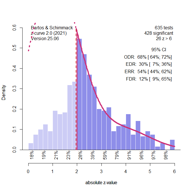
Visual inspection of the z-curve plot shows evidence of selection bias. This is confirmed by a comparison of the ODR (68%) and the 95%CI of the EDR, 7% to 36%. There are too many significant results. The higher ERR (54%) than ERR (30%) also provides evidence of heterogeneity. A direct test of heterogeneity further confirms this finding. The model with one-component and a fixed SD of 1 did not fit the data as well as a model with 1 component and a free SD parameter, one-sided 95%CI = .021. The 95%CI for the SD parameter ranged from 1.82 to 2.25. The two-component model fit the data slightly better than the one-component model with a free SD, suggesting that the distribution of z-values is not normal.

The EDR and EER estimates translate into the following effect size estimates. For all positive results, the average effect size estimate is d = .42, 95%CI = .14 to .49. This is considerably lower than the estimate with the 3PSM model. For positive and significant results, the estimate is d = .61, 95%CI = .53 to .67. This estimate is very close to the p-uniform estimate.

In conclusion, while it is difficult to provide a precise estimate of the average effect size for all studies that have been conducted, including many studies that were never reported, the 3PSM model, p-uniform, and z-curve all agree that positive results and positive significant results were obtained with a moderate to large effect size. The PET-PEESE results are irrelevant because the overall average is not informative in the presence of large heterogeneity. This conclusion is consistent with Cheng et al.’s (2025) discussion of their results that emphasizes “extremely wide range of possible effect sizes arising from differences in study design” (p. 18). Thye even consider it possible that effect sizes of -1 are plausible, although they imply that researchers can obtain strong results that contradict theoretical predictions.

At the same time, Cheng et al. (2025) claim that many terror management studies are underpowered. This claim seems inconsistent with the ERR estimate that studies with significant results have 54% power for studies with significant results. It is also inconsistent with the finding that these studies, on average, have a strong positive effect. The claim that studies are underpowered is based on Cheng et al.’s (2025) p-curve and z-curve analysis that used a different dataset than the dataset that was used for effect size estimation. For this dataset, p-curve estimated 25% power and z-curve estimated an ERR of 19%. Transforming power estimates into effect size estimates and vice versa reveals that the two datasets lead to inconsistent conclusions about the terror management literature.

To use the data for effect size estimation, I limited the set of studies to two-group designs with t-tests or F-tests with one-degree of freedom. The latter results can be transformed into t-values by computing the square root of the F-value. I also deleted the few studies with negative results.

The p-curve estimate of 25% power translates into an effect size estimate for positive and significant studies of d = .30. The figure shows the new z-curve results for this dataset. The ERR estimate is similar to the ERR estimate in the published article (20% vs. 18%). The EDR estimates is higher (18% vs. 8%), but not significantly so, given the wide confidence interval around this estimate. The z-curve effect size estimate for positive and significant studies was similar to the p-curve estimate, d = .26, 95%CI = .20 to .31. The z-curve estimate for studies with positive results based on the EDR was d = .24, with a wider confidence interval ranging from d = .00 to .28. These estimates are notably lower than those based on the first dataset.

A comparison of the z-curve plot shows the main difference between the two datasets. Whereas the first dataset has a long tail of studies with strong evidence (z > 4, including 26 results with z > 6), the second dataset has few studies with strong evidence (z > 4) and only 10 studies with z-scores greater than 6.

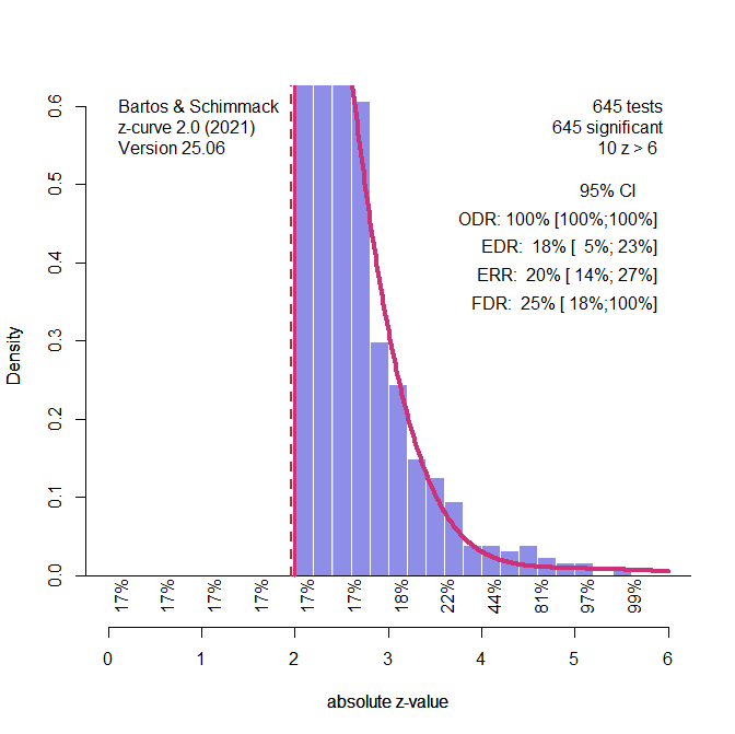
This difference also implies less heterogeneity in the second dataset. Without heterogeneity, the EDR and ERR estimates are bound to be similar. The direct test of heterogeneity also shows little evidence of heterogeneity in power. The one-sided 95%CI for the difference test of fit was .00 for both tests and the 95%CI for the free SD parameter ranged from 1.00 to 1.09. In short, z-curve shows less heterogeneity in power, lower average power, and smaller effect size estimates for Cheng et al.’s (2025) p-curve dataset than for their effect-size meta-analysis dataset.

The p-uniform estimate was in line with the z-curve estimate for positive and significant results, d = .29, 95%CI = .25 to .32.

The 3PSM model produced a lower estimate of the average effect, d = .10, 95%CI = .07 to .13, but it found evidence of small heterogeneity, tau = .25, 95%CI = .22 to .28. Thus, the estimated effect size for only positive results is higher, d = .21 and in line with the z-curve estimate. And the average effect for positive and significant results is d = .36, which is in line with z-curve and p-uniform estimates.

The PET regression produced a non-significant estimate of d = .01, 95%CI = -.04 to .06. The PEESE estimate is d = .27, 95%CI = .24 to .30. Based on the PET-PEESE logic, the PET estimate is the best estimate of the overall effect size. If studies are heterogenous in effect sizes, this implies a positive effect for studies with positive results, but PET-PEESE does not provide an effect size estimate that can be compared to the other methods.

In conclusion, p-curve, z-curve, p-uniform, and the 3PSM model produced consistent results when the same dataset was analyzed. All methods suggest that studies with a positive result have a small average effect size. Z-curve finds no evidence of heterogeneity in power, while 3PSM finds small heterogeneity in effect sizes. This is not necessarily inconsistent if there is a negative correlation between population effect sizes and sampling error (that is researchers use larger samples when they expect weaker effects).

These results are notably different from those obtained with the first dataset. Thus, Cheng et al.’s (2025) conflicting results are due to the analyze of different datasets rather than inconsistent results of different meta-analytic methods. For applied researchers, the most interesting finding is that the first dataset contains a larger set of studies with strong evidence. These studies may help to find the proverbial needle of replicable results in the pile of p-hacked significant results.

General Discussion

Meta-science is not fundamentally different from other sciences. Just like original researchers, meta-scientists have ample degrees of freedom when they conduct their empirical studies. In the old days, these degrees of freedom were often exploited to present desired results. For example, some meta-analysis did not report results of bias tests or correct for publication bias when it was present (). Fortunately, these days are over, and it is becoming more common to report the results of various meta-analytic tools that make different assumptions and require different data as input (e.g., effect sizes vs. z-values). While multiverse analyses have the advantage of transparency, they also confuse researchers and readers unfamiliar with new methods.

I hope that my detailed examination of two multiverse meta-analysis clarifies some of the confusion and helps researchers to draw the proper conclusions from their data. First, I showed that it is possible and important to test assumption about publication bias and heterogeneity. While the slope in PET-PEESE can suggest the presence of publication bias, the evidence is ambiguous because other factors could produce this relationship. Therefore, election models like 3PSM and z-curve are superior methods to examine the presence of selection bias. Both methods also test for heterogeneity in the data. While the direct test of heterogeneity with z-curve is new and requires some validation work, the difference between the EDR and ERR provides some information about heterogeneity because selection for significance with heterogeneity increases the ERR. Researchers who are skeptical about z-curve need to rely on 3PSM to examine heterogeneity in effect sizes.

Applied researchers struggle with the interpretation of meta-analytic results when heterogeneity is present. Maybe this problem is caused by a strong focus on average effects in psychology. Heterogeneity across individuals is not unlike personality differences in original studies. On average, people are neither extraverted, nor introverted, but half the population is more extraverted and the other half is more introverted. The average is hardly of interest. The same is true for an average effect size of zero, when heterogeneity is present. The average does not mean that there are no notable effects. It implies that half the studies have a positive effect and the other half have a negative effect. The next step is to examine moderators that explain these differences.

Discussion of heterogeneity in effect sizes suggests some confusion about the meaning of negative effect sizes. For example, Cheng et al. (2025) correctly point out that the large tau parameter in their 3PSM analysis suggests that population effect sizes can range from -1.05 to 1.77 without pointing out that a negative effect of d = -1.00 implies that an effect is in the opposite direction that is suggested by theory. For example, let’s assume that fear of death is supposed to make people focus more on meaning than pleasure in life. An effect size of d = -1.00 would imply that the researchers found a strong effect in the opposite direction. However, they do not reverse the hypothesis after the fact (HARKing) and conclude that their hypothesis was not supported. Everybody who has read a fair share of articles knows that this never happens. Indeed, the dataset contains less than 1% surprising findings with a significant negative effect. The problem here is that the 3PSM model assumes normal distribution of population effect sizes. If it finds strong heterogeneity among positive results, the tau parameter inevitable suggests that there are also negative results without any evidence to back this up. It is therefore best to ignore this prediction and to compute the implied average effect size for positive results that is implied by the model parameters. As shown, these results are similar to z-curve results and have the advantage that the estimate applies to the effects that were actually observed rather than an imaginary set of studies with negative results.

There is also confusion about the interpretation of results from models that focus on positive and statistically significant results like p-uniform. For example, Carter et al. (2019) concluded that p-uniform produces large type-I error rates when data are heterogenous. This is a misinterpretation of the results because heterogeneity implies that positive and significant results have a non-zero average. It is therefore false to use the overall average of zero as a criterion for p-uniform. This is also true for z-curve estimates for all positive results and all negative results. When heterogeneity is present, the averages are greater than zero by definition even if the overall average is zero or negative. It is therefore important to specify clearly the population of studies that are of interest. The overall average of all studies is rarely of interest, especially when strong publication bias is present. Who cares how many studies with no effect or weak effects were conducted and never published. The real question is whether the published studies with significant results provide credible evidence for an effect and what the effect size might be after we take selection for significance into account. The inclusion of non-significant results only makes sense when studies examine the same question, like in clinical trials with a clear intervention and outcome. That is, studies are direct replications of each other. When studies differ in designs, outcome variables and other characteristics, a focus on studies that really worked makes more sense. That is, when studies are conceptual replications and publication bias is present, the first question is whether some studies did produce credible evidence for a practically significant effect.

The most surprising finding in this meta-meta-analysis was the variation of results as a function of data rather than methods. Typical effect size coding produces large heterogeneity and a subset of studies with large effects. Coding of focal hypothesis produces more homogenous results and less evidence of real effects. More attention needs to be paid to this part of meta-analysis. The influence of coding on results was only observed by applying all methods to the same dataset. This requires just a few transformations of effect sizes into test statistics or test-statistics into effect sizes. There is no need to code studies differently for different meta-analytic methods. Power based estimates with p-curve (not recommended) or z-curve can be easily converted into effect sizes to make the results more comparable with the results of other methods. The code to perform similar analysis on new datasets s available on OSF.

References

Bartoš, F., Maier, M., Quintana, D. S., & Wagenmakers E.-J. Adjusting for Publication Bias in JASP and R: Selection Models, PET-PEESE, and Robust Bayesian Meta-Analysis. Advances in Methods and Practices in Psychological Science. 2022;5(3). doi:10.1177/25152459221109259

Bartoš, F., & Schimmack, U. (2022). Z-curve 2.0: Estimating replication rates and discovery rates. Meta-Psychology, 6, Article e0000130. https://doi.org/10.15626/MP.2022.2981

Brunner, J., & Schimmack, U. (2020). Estimating population mean power under conditions of heterogeneity and selection for significance. Meta- Psychology. MP.2018.874, https://doi.org/10.15626/MP.2018.874

Carter E. C., Schönbrodt, F. D., Gervais, W. M., Hilgard, J. (2019). Correcting for Bias in Psychology: A Comparison of Meta-Analytic Methods. Advances in Methods and Practices in Psychological Science. 2019;2(2):115-144. doi:10.1177/2515245919847196

Chen, L., Benjamin, R., Guo, Y., Lai, A., & Heine, S. J. (2025). Managing the terror of publication bias: A systematic review of the mortality salience hypothesis. Journal of Personality and Social Psychology. Advance online publication. https://dx.doi.org/10.1037/pspa0000438

Fanelli, D. (2011). Negative results are disappearing from most disciplines and countries. Scientometrics, 90, 891–904.

Maier, M., Bartoš, F., & Wagenmakers, E.-J. (2022). Robust Bayesian meta-analysis: Addressing publication bias with model-averaging. Psychological Methods, 27(5), 723–743.
https://doi.org/10.1037/met0000476

Open Science Collaboration (OSC). (2015). Estimating the reproducibility of psychological science. Science, 349, aac4716. http://dx.doi.org/10.1126/science.aac4716

Sterling, T. D., Rosenbaum, W. L., & Weinkam, J. J. (1995). Publication decisions revisited: The effect of the outcome of statistical tests on the decision to publish and vice versa. The American Statistician, 49, 108–112