Tag Archives: replicability

Replicability-Ranking of 100 Social Psychology Departments

Please see the new post on rankings of psychology departments that is based on all areas of psychology and covers the years from 2010 to 2015 with separate information for the years 2012-2015.

===========================================================================

Old post on rankings of social psychology research at 100 Psychology Departments

This post provides the first analysis of replicability for individual departments. The table focuses on social psychology and the results cannot be generalized to other research areas in the same department. An explanation of the rational and methodology of replicability rankings follows in the text below the table.

Department 2010-2014
Macquarie University 91
New Mexico State University 82
The Australian National University 81
University of Western Australia 74
Maastricht University 70
Erasmus University Rotterdam 70
Boston University 69
KU Leuven 67
Brown University 67
University of Western Ontario 67
Carnegie Mellon 67
Ghent University 66
University of Tokyo 64
University of Zurich 64
Purdue University 64
University College London 63
Peking University 63
Tilburg University 63
University of California, Irvine 63
University of Birmingham 62
University of Leeds 62
Victoria University of Wellington 62
University of Kent 62
Princeton 61
University of Queensland 61
Pennsylvania State University 61
Cornell University 59
University of California at Los Angeles 59
University of Pennsylvania 59
University of New South Wales (UNSW) 59
Ohio State University 58
National University of Singapore 58
Vanderbilt University 58
Humboldt Universit„ät Berlin 58
Radboud University 58
University of Oregon 58
Harvard University 56
University of California, San Diego 56
University of Washington 56
Stanford University 55
Dartmouth College 55
SUNY Albany 55
University of Amsterdam 54
University of Texas, Austin 54
University of Hong Kong 54
Chinese University of Hong Kong 54
Simone Fraser University 54
Ruprecht-Karls-Universitaet Heidelberg 53
University of Florida 53
Yale University 52
University of California, Berkeley 52
University of Wisconsin 52
University of Minnesota 52
Indiana University 52
University of Maryland 52
University of Toronto 51
Northwestern University 51
University of Illinois at Urbana-Champaign 51
Nanyang Technological University 51
University of Konstanz 51
Oxford University 50
York University 50
Freie Universit„ät Berlin 50
University of Virginia 50
University of Melbourne 49
Leiden University 49
University of Colorado, Boulder 49
Univeritä„t Würzburg 49
New York University 48
McGill University 48
University of Kansas 48
University of Exeter 47
Cardiff University 46
University of California, Davis 46
University of Groningen 46
University of Michigan 45
University of Kentucky 44
Columbia University 44
University of Chicago 44
Michigan State University 44
University of British Columbia 43
Arizona State University 43
University of Southern California 41
Utrecht University 41
University of Iowa 41
Northeastern University 41
University of Waterloo 40
University of Sydney 40
University of Bristol 40
University of North Carolina, Chapel Hill 40
University of California, Santa Barbara 40
University of Arizona 40
Cambridge University 38
SUNY Buffalo 38
Duke University 37
Florida State University 37
Washington University, St. Louis 37
Ludwig-Maximilians-Universit„ät München 36
University of Missouri 34
London School of Economics 33

Replicability scores of 50% and less are considered inadequate (grade F). The reason is that less than 50% of the published results are expected to produce a significant result in a replication study, and with less than 50% successful replications, the most rational approach is to treat all results as false because it is unclear which results would replicate and which results would not replicate.

RATIONALE AND METHODOLOGY

University rankings have become increasingly important in science. Top ranking universities use these rankings to advertise their status. The availability of a single number of quality and distinction creates pressures on scientists to meet criteria that are being used for these rankings. One key criterion is the number of scientific articles that are being published in top ranking scientific journals under the assumption that these impact factors of scientific journals track the quality of scientific research. However, top ranking journals place a heavy premium on novelty without ensuring that novel findings are actually true discoveries. Many of these high-profile discoveries fail to replicate in actual replication studies. The reason for the high rate of replication failures is that scientists are rewarded for successful studies, while there is no incentive to publish failures. The problem is that many of these successful studies are obtained with the help of luck or questionable research methods. For example, scientists do not report studies that fail to support their theories. The problem of bias in published results has been known for a long time (Sterling, 1959). However, few researchers were aware of the extent of the problem.   New evidence suggests that more than half of published results provide false or extremely biased evidence. When more than half of published results are not credible, a science loses its credibility because it is not clear which results can be trusted and which results provide false information.

The credibility and replicability of published findings varies across scientific disciplines (Fanelli, 2010). More credible sciences are more willing to conduct replication studies and to revise original evidence. Thus, it is inappropriate to make generalized claims about the credibility of science. Even within a scientific discipline credibility and replicability can vary across sub-disciplines. For example, results from cognitive psychology are more replicable than results from social psychology. The replicability of social psychological findings is extremely low. Despite an increase in sample size, which makes it easier to obtain a significant result in a replication study, only 5 out of 38 replication studies produced a significant result. If the replication studies had used the same sample sizes as the original studies, only 3 out of 38 results would have replicated, that is, produced a significant result in the replication study. Thus, most published results in social psychology are not trustworthy.

There have been mixed reactions by social psychologists to the replication crisis in social psychology. On the one hand, prominent leaders of the field have defended the status quo with the following arguments.

1 – The experiments who conducted the replication studies are incompetent (Bargh, Schnall, Gilbert).

2 – A mysterious force makes effects disappear over time (Schooler).

3 – A statistical artifact (regression to the mean) will always make it harder to find significant results in a replication study (Fiedler).

4 – It is impossible to repeat social psychological studies exactly and a replication study is likely to produce different results than an original study (the hidden moderator) (Schwarz, Strack).

These arguments can be easily dismissed because they do not explain why cognitive psychologists and other scientific disciplines have more successful replications and more failed results.   The real reason for the low replicability of social psychology is that social psychologists conduct many, relatively cheap studies that often fail to produce the expected results. They then conduct exploratory data analyses to find unexpected patterns in the data or they simply discard the study and publish only studies that support a theory that is consistent with the data (Bem). This hazardous approach to science can produce false positive results. For example, it allowed Bem (2011) to publish 9 significant results that seemed to show that humans can foresee unpredictable outcomes in the future. Some prominent social psychologists defend this approach to science.

“We did run multiple studies, some of which did not work, and some of which worked better than others. You may think that not reporting the less successful studies is wrong, but that is how the field works.” (Roy Baumeister,)

The lack of rigorous scientific standards also allowed Diederik Stapel, a prominent social psychologist to fabricate data, which led to over 50 retractions of scientific articles. The commission that investigated Stapel came to the conclusion that he was only able to publish so many fake articles because social psychology is a “sloppy science,” where cute findings and sexy stories count more than empirical facts.

Social psychology faces a crisis of confidence. While social psychology tried hard to convince the general public that it is a real science, it actually failed to follow standard norms of science to ensure that social psychological theories are based on objective replicable findings. Social psychology therefore needs to reform its practices if it wants to be taken serious as a scientific field that can provide valuable insights into important question about human nature and human behavior.

There are many social psychologists who want to improve scientific standards. For example, the head of the OSF-reproducibility project, Brian Nosek, is a trained social psychologist. Mickey Inzlicht published a courageous self-analysis that revealed problems in some of his most highly cited articles and changed the way his lab is conducting studies to improve social psychology. Incoming editors of social psychology journals are implementing policies to increase the credibility of results published in their journals (Simine Vazire; Roger Giner-Sorolla). One problem for social psychologists willing to improve their science is that the current incentive structure does not reward replicability. The reason is that it is possible to count number of articles and number of citations, but it seems difficult to quantify replicability and scientific integrity.

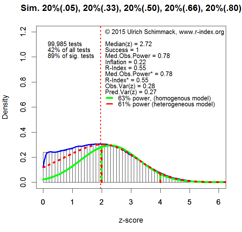
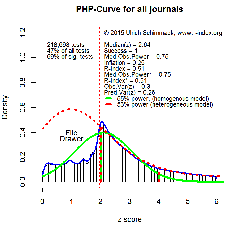
To address this problem, Jerry Brunner and I developed a quantitative measure of replicability. The replicability-score uses published statistical results (p-values) and transforms them into absolute z-scores. The distribution of z-scores provides information about the statistical power of a study given the sample size, design, and observed effect size. Most important, the method takes publication bias into account and can estimate the true typical power of published results. It also reveals the presence of a file-drawer of unpublished failed studies, if the published studies contain more significant results than the actual power of studies allows. The method is illustrated in the following figure that is based on t- and F-tests published in the most important journals that publish social psychology research.

PHP-Curve Social Journals

The green curve in the figure illustrates the distribution of z-scores that would be expected if a set of studies had 53% power. That is, random sampling error will sometimes inflate the observed effect size and sometimes deflate the observed effect size in a sample relative to the population effect size. With 54% power, there would be 46% (1 – .54 = .46) non-significant results because the study had insufficient power to demonstrate an effect that actually exists. The graph shows that the green curve fails to describe the distribution of observed z-scores. On the one hand, there are more extremely high z-scores. This reveals that the set of studies is heterogeneous. Some studies had more than 54% power and others had less than 54% power. On the other hand, there are fewer non-significant results than the green curve predicts. This discrepancy reveals that non-significant results are omitted from the published reports.

Given the heterogeneity of true power, the red curve is more appropriate. It provides the best fit to the observed z-scores that are significant (z-scores > 2). It does not model the z-scores below 2 because non-significant z-scores are not reported.   The red-curve gives a lower estimate of power and shows a much larger file-drawer.

I limit the power analysis to z-scores in the range from 2 to 4. The reason is that z-scores greater than 4 imply very high power (> 99%). In fact, many of these results tend to replicate well. However, many theoretically important findings are published with z-scores less than 4 as evidence. These z-scores do not replicate well. If social psychology wants to improve its replicability, social psychologists need to conduct fewer studies with more statistical power that yield stronger evidence and they need to publish all studies to reduce the file-drawer.

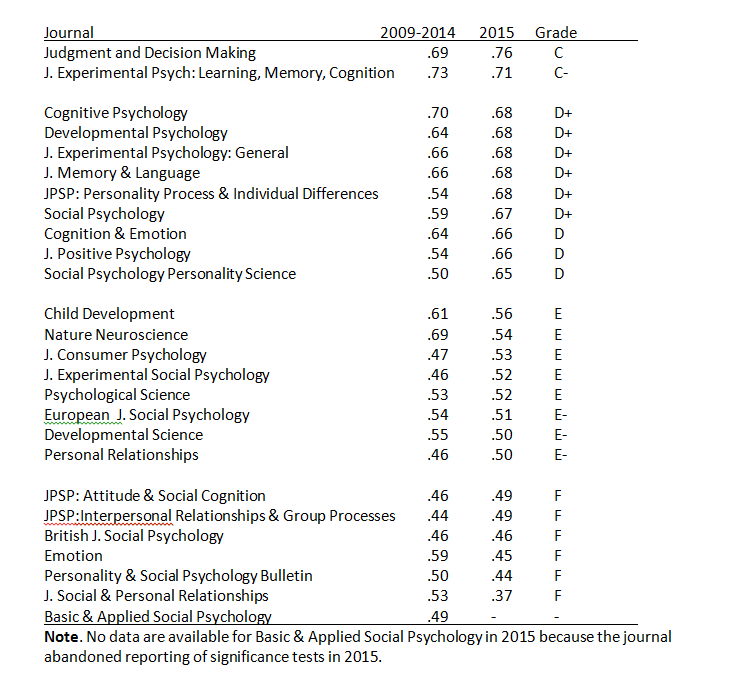
To provide an incentive to increase the scientific standards in social psychology, I computed the replicability-score (homogeneous model for z-scores between 2 and 4) for different journals. Journal editors can use the replicability rankings to demonstrate that their journal publishes replicable results. Here I report the first rankings of social psychology departments.   To rank departments, I searched the database of articles published in social psychology journals for the affiliation of articles’ authors. The rankings are based on the z-scores of these articles published in the years 2010 to 2014. I also conducted an analysis for the year 2015. However, the replicability scores were uncorrelated with those in 2010-2014 (r = .01). This means that the 2015 results are unreliable because the analysis is based on too few observations. As a result, the replicability rankings of social psychology departments cannot reveal recent changes in scientific practices. Nevertheless, they provide a first benchmark to track replicability of psychology departments. This benchmark can be used by departments to monitor improvements in scientific practices and can serve as an incentive for departments to create policies and reward structures that reward scientific integrity over quantitative indicators of publication output and popularity. Replicabilty is only one aspect of high-quality research, but it is a necessary one. Without sound empirical evidence that supports a theoretical claim, discoveries are not real discoveries.

Examining the Replicability of 66,212 Published Results in Social Psychology: A Post-Hoc-Power Analysis Informed by the Actual Success Rate in the OSF-Reproducibilty Project

The OSF-Reproducibility-Project examined the replicability of 99 statistical results published in three psychology journals. The journals covered mostly research in cognitive psychology and social psychology. An article in Science, reported that only 35% of the results were successfully replicated (i.e., produced a statistically significant result in the replication study).

I have conducted more detailed analyses of replication studies in social psychology and cognitive psychology. Cognitive psychology had a notably higher success rate (50%, 19 out of 38) than social psychology (8%, 3 out of 38). The main reason for this discrepancy is that social psychologists and cognitive psychologists use different designs. Whereas cognitive psychologists typically use within-subject designs with many repeated measurements of the same individual, social psychologists typically assign participants to different groups and compare behavior on a single measure. This so-called between-subject design makes it difficult to detect small experimental effects because it does not control the influence of other factors that influence participants’ behavior (e.g., personality dispositions, mood, etc.). To detect small effects in these noisy data, between-subject designs require large sample sizes.

It has been known for a long time that sample sizes in between-subject designs in psychology are too small to have a reasonable chance to detect an effect (less than 50% chance to find an effect that is actually there) (Cohen, 1962; Schimmack, 2012; Sedlmeier & Giegerenzer, 1989). As a result, many studies fail to find statistically significant results, but these studies are not submitted for publication. Thus, only studies that achieved statistical significance with the help of chance (the difference between two groups is inflated by uncontrolled factors such as personality) are reported in journals. The selective reporting of lucky results creates a bias in the published literature that gives a false impression of the replicability of published results. The OSF-results for social psychology make it possible to estimate the consequences of publication bias on the replicability of results published in social psychology journals.

A naïve estimate of the replicability of studies would rely on the actual success rate in journals. If journals would publish significant and non-significant results, this would be a reasonable approach. However, journals tend to publish exclusively significant results. As a result, the success rate in journals (over 90% significant results; Sterling, 1959; Sterling et al., 1995) gives a drastically inflated estimate of replicability.

A somewhat better estimate of replicability can be obtained by computing post-hoc power based on the observed effect sizes and sample sizes of published studies. Statistical power is the long-run probability that a series of exact replication studies with the same sample size would produce significant results. Cohen (1962) estimated that the typical power of psychological studies is about 60%. Thus, even for 100 studies that all reported significant results, only 60 are expected to produce a significant result again in the replication attempt.

The problem with Cohen’s (1962) estimate of replicability is that post-hoc-power analysis uses the reported effect sizes as an estimate of the effect size in the population. However, due to the selection bias in journals, the reported effect sizes and power estimates are inflated. In collaboration with Jerry Brunner, I have developed an improved method to estimate typical power of reported results that corrects for the inflation in reported effect sizes. I applied this method to results from 38 social psychology articles included in the OSF-reproducibility project and obtained a replicability estimate of 35%.

The OSF-reproducbility project provides another opportunity to estimate the replicability of results in social psychology. The OSF-project selected a representative set of studies from two journals and tried to reproduce the same experimental conditions as closely as possible. This should produce unbiased results and the success rate provides an estimate of replicability. The advantage of this method is that it does not rely on statistical assumptions. The disadvantage is that the success rate depends on the ability to exactly recreate the conditions of the original studies. Any differences between studies (e.g., recruiting participants from different populations) can change the success rate. The OSF replication studies also often changed the sample size of the replication study, which will also change the success rate. If sample sizes in a replication study are larger, power increases and the success rate no longer can be used as an estimate of the typical replicability of social psychology. To address this problem, it is possible to apply a statistical adjustment and use the success rate that would have occurred with the original sample sizes. I found that 5 out of 38 (13%) produced significant results and after correcting for the increase in sample size, replicability was only 8% (3 out of 38).

One important question is how how representative the 38 results from the OSF-project are for social psychology in general. Unfortunately, it is practically impossible and too expensive to conduct a large number of exact replication studies. In comparison, it is relatively easy to apply post-hoc power analysis to a large number of statistical results reported in social psychology. Thus, I examined the representativeness of the OSF-reproducibility results by comparing the results of my post-hoc power analysis based on the 38 results in the OSF to a post-hoc-power analysis of a much larger number of results reported in major social psychology journals .

I downloaded articles from 12 social psychology journals, which are the primary outlets for publishing experimental social psychology research: Basic and Applied Social Psychology, British Journal of Social Psychology, European Journal of Social Psychology, Journal of Experimental Social Psychology, Journal of Personality and Social Psychology: Attitudes and Social Cognition, Journal of Personality and Social Psychology: Interpersonal Relationships and Group Processes, Journal of Social and Personal Relationships, Personal Relationships, Personality and Social Psychology Bulletin, Social Cognition, Social Psychology and Personality Science, Social Psychology.

I converted pdf files into text files and searched for all reports of t-tests or F-tests and converted the reported test-statistic into exact two-tailed p-values. The two-tailed p-values were then converted into z-scores by finding the z-score corresponding to the probability of 1-p/2, with p equal the two-tailed p-value. The total number of z-scores included in the analysis is 134,929.

I limited my estimate of power to z-scores in the range between 2 and 4. Z-scores below 2 are not statistically significant (z = 1.96, p = .05). Sometimes these results are reported as marginal evidence for an effect, sometimes they are reported as evidence that an effect is not present, and sometimes they are reported without an inference about the population effect. It is more important to determine the replicability of results that are reported as statistically significant support for a prediction. Z-scores greater than 4 were excluded because z-scores greater than 4 imply that this test had high statistical power (> 99%). Many of these results replicated successfully in the OSF-project. Thus, a simple rule is to assign a success rate of 100% to these findings. The Figure below shows the distribution of z-scores in the range form z = 0 to6, but the power estimate is applied to z-scores in the range between 2 and 4 (n = 66,212).

The power estimate based on the post-hoc-power curve for z-scores between 2 and 4 is 46%. It is important to realize that this estimate is based on 70% of all significant results that were reported. As z-scores greater than 4 essentially have a power of 100%, the overall power estimate for all statistical tests that were reported is .46*.70 + .30 = .62. It is also important to keep in mind that this analysis uses all statistical tests that were reported including manipulation checks (e.g., pleasant picture were rated as more pleasant than unpleasant pictures). For this reason, the range of z-scores is limited to values between 2 and 4, which is much more likely to reflect a test of a focal hypothesis.

46% power for z-scores between 2 and 4 of is a higher estimate than the estimate for the 38 studies in the OSF-reproducibility project (35%). This suggests that the estimated replicability based on the OSF-results is an underestimation of the true replicability. The discrepancy between predicted and observed replicability in social psychology (8 vs. 38) and cognitive psychology (50 vs. 75), suggests that the rate of actual successful replications is about 20 to 30% lower than the success rate based on statistical prediction. Thus, the present analysis suggests that actual replication attempts of results in social psychology would produce significant results in about a quarter of all attempts (46% – 20% = 26%).

The large sample of test results makes it possible to make more detailed predictions for results with different strength of evidence. To provide estimates of replicability for different levels of evidence, I conducted post-hoc power analysis for intervals of half a standard deviation (z = .5). The power estimates are:

Strength of Evidence      Power    

2.0 to 2.5                            33%

2.5 to 3.0                            46%

3.0 to 3.5                            58%

3.5 to 4.0                            72%

IMPLICATIONS FOR PLANNING OF REPLICATION STUDIES

These estimates are important for researchers who are aiming to replicate a published study in social psychology. The reported effect sizes are inflated and a replication study with the same sample size has a low chance to produce a significant result even if a smaller effect exists.   To conducted a properly powered replication study, researchers would have to increase sample sizes. To illustrate, imagine that a study demonstrate a significant difference between two groups with 40 participants (20 in each cell) with a z-score of 2.3 (p = .02, two-tailed). The observed power for this result is 65% and it would suggest that a slightly larger sample of N = 60 is sufficient to achieve 80% power (80% chance to get a significant result). However, after correcting for bias, the true power is more likely to be just 33% (see table above) and power for a study with N = 60 would still only be 50%. To achieve 80% power, the replication study would need a sample size of 130 participants. Sample sizes would need to be even larger taking into account that the actual probability of a successful replication is even lower than the probability based on post-hoc power analysis. In the OSF-project only 1 out of 30 studies with an original z-score between 2 and 3 was successfully replicated.

IMPLICATIONS FOR THE EVALUATION OF PUBLISHED RESULTS

The results also have implications for the way social psychologists should conduct and evaluate new research. The main reason why z-scores between 2 and 3 provide untrustworthy evidence for an effect is that they are obtained with underpowered studies and publication bias. As a result, it is likely that the strength of evidence is inflated. If, however, the same z-scores were obtained in studies with high power, a z-score of 2.5 would provide more credible evidence for an effect. The strength of evidence in a single study would still be subject to random sampling error, but it would no longer be subject to systematic bias. Therefore, the evidence would be more likely to reveal a true effect and it would be less like to be a false positive.   This implies that z-scores should be interpreted in the context of other information about the likelihood of selection bias. For example, a z-score of 2.5 in a pre-registered study provides stronger evidence for an effect than the same z-score in a study where researchers may have had a chance to conduct multiple studies and to select the most favorable results for publication.

The same logic can also be applied to journals and labs. A z-score of 2.5 in a journal with an average z-score of 2.3 is less trustworthy than a z-score of 2.5 in a journal with an average z-score of 3.5. In the former journal, a z-score of 2.5 is likely to be inflated, whereas in the latter journal a z-score of 2.5 is more likely to be negatively biased by sampling error. For example, currently a z-score of 2.5 is more likely to reveal a true effect if it is published in a cognitive journal than a social journal (see ranking of psychology journals).

The same logic applies even more strongly to labs because labs have a distinct research culture (MO). Some labs conduct many underpowered studies and publish only the studies that worked. Other labs may conduct fewer studies with high power. A z-score of 2.5 is more trustworthy if it comes from a lab with high average power than from a lab with low average power. Thus, providing information about the post-hoc-power of individual researchers can help readers to evaluate the strength of evidence of individual studies in the context of the typical strength of evidence that is obtained in a specific lab. This will create an incentive to publish results with strong evidence rather than fishing for significant results because a low replicability index increases the criterion at which results from a lab provide evidence for an effect.

The Replicability of Social Psychology in the OSF-Reproducibility Project

Abstract:  I predicted the replicability of 38 social psychology results in the OSF-Reproducibility Project. Based on post-hoc-power analysis I predicted a success rate of 35%.  The actual success rate was 8% (3 out of 38) and post-hoc-power was estimated to be 3% for 36 out of 38 studies (5% power = type-I error rate, meaning the null-hypothesis is true).

The OSF-Reproducibility Project aimed to replicate 100 results published in original research articles in three psychology journals in 2008. The selected journals focus on publishing results from experimental psychology. The main paradigm of experimental psychology is to recruit samples of participants and to study their behaviors in controlled laboratory conditions. The results are then generalized to the typical behavior of the average person.

An important methodological distinction in experimental psychology is the research design. In a within-subject design, participants are exposed to several (a minimum of two) situations and the question of interest is whether responses to one situation differ from behavior in other situations. The advantage of this design is that individuals serve as their own controls and variation due to unobserved causes (mood, personality, etc.) does not influence the results. This design can produce high statistical power to study even small effects. The design is often used by cognitive psychologists because the actual behaviors are often simple behaviors (e.g., pressing a button) that can be repeated many times (e.g., to demonstrate interference in the Stroop paradigm).

In a between-subject design, participants are randomly assigned to different conditions. A mean difference between conditions reveals that the experimental manipulation influenced behavior. The advantage of this design is that behavior is not influenced by previous behaviors in the experiment (carry over effects). The disadvantage is that many uncontrolled factors (e..g, mood, personality) also influence behavior. As a result, it can be difficult to detect small effects of an experimental manipulation among all of the other variance that is caused by uncontrolled factors. As a result, between-subject designs require large samples to study small effects or they can only be used to study large effects.

One of the main findings of the OSF-Reproducibility Project was that results from within-subject designs used by cognitive psychology were more likely to replicate than results from between-subject designs used by social psychologists. There were two few between-subject studies by cognitive psychologists or within-subject designs by social psychologists to separate these factors.   This result of the OSF-reproducibility project was predicted by PHP-curves of the actual articles as well as PHP-curves of cognitive and social journals (Replicability-Rankings).

Given the reliable difference between disciplines within psychology, it seems problematic to generalize the results of the OSF-reproducibility project to all areas of psychology. The Replicability-Rankings suggest that social psychology has a lower replicability than other areas of psychology. For this reason, I conducted separate analyses for social psychology and for cognitive psychology. Other areas of psychology had two few studies to conduct a meaningful analysis. Thus, the OSF-reproducibility results should not be generalized to all areas of psychology.

The master data file of the OSF-reproducibilty project contained 167 studies with replication results for 99 studies.   57 studies were classified as social studies. However, this classification used a broad definition of social psychology that included personality psychology and developmental psychology. It included six articles published in the personality section of the Journal of Personality and Social Psychology. As each section functions essentially like an independent journal, I excluded all studies from this section. The file also contained two independent replications of two experiments (experiment 5 and 7) in Albarracín et al. (2008; DOI: 10.1037/a0012833). As the main sampling strategy was to select the last study of each article, I only included Study 7 in the analysis (Study 5 did not replicate, p = .77). Thus, my selection did not lower the rate of successful replications. There were also two independent replications of the same result in Bressan and Stranieri (2008). Both replications produced non-significant results (p = .63, p = .75). I selected the replication study with the larger sample (N = 318 vs. 259). I also excluded two studies that were not independent replications. Rule and Ambady (2008) examined the correlation between facial features and success of CEOs. The replication study had new raters to rate the faces, but used the same faces. Heine, Buchtel, and Norenzayan (2008) examined correlates of conscientiousness across nations and the replication study examined the same relationship across the same set of nations. I also excluded replications of non-significant results because non-significant results provide ambiguous information and cannot be interpreted as evidence for the null-hypothesis. For this reason, it is not clear how the results of a replication study should be interpreted. Two underpowered studies could easily produce consistent results that are both type-II errors. For this reason, I excluded Ranganath and Nosek (2008) and Eastwick and Finkel (2008). The final sample consisted of 38 articles.

I first conducted a post-hoc-power analysis of the reported original results. Test statistics were first converted into two-tailed p-values and two-tailed p-values were converted into absolute z-scores using the formula (1 – norm.inverse(1-p/2). Post-hoc power was estimated by fitting the observed z-scores to predicted z-scores with a mixed-power model with three parameters (Brunner & Schimmack, in preparation).

Estimated power was 35%. This finding reflects the typical finding that reported results are a biased sample of studies that produced significant results, whereas non-significant results are not submitted for publication. Based on this estimate, one would expect that only 35% of the 38 findings (k = 13) would produce a significant result in an exact replication study with the same design and sample size.

The Figure visualizes the discrepancy between observed z-scores and the success rate in the original studies. Evidently, the distribution is truncated and the mode of the curve (it’s highest point) is projected to be on the left side of the significance criterion (z = 1.96, p = .05 (two-tailed)). Given the absence of reliable data in the range from 0 to 1.96, the data make it impossible to estimate the exact distribution in this region, but the step decline of z-scores on the right side of the significance criterion suggests that many of the significant results achieved significance only with the help of inflated observed effect sizes. As sampling error is random, these results will not replicate again in a replication study.

The replication studies had different sample sizes than the original studies. This makes it difficult to compare the prediction to the actual success rate because the actual success rate could be much higher if the replication studies had much larger samples and more power to replicate effects. For example, if all replication studies had sample sizes of N = 1,000, we would expect a much higher replication rate than 35%. The median sample size of the original studies was N = 86. This is representative of studies in social psychology. The median sample size of the replication studies was N = 120. Given this increase in power, the predicted success rate would increase to 50%. However, the increase in power was not uniform across studies. Therefore, I used the p-values and sample size of the replication study to compute the z-score that would have been obtained with the original sample size and I used these results to compare the predicted success rate to the actual success rate in the OSF-reproducibility project.

The depressing finding was that the actual success rate was much lower than the predicted success rate. Only 3 out of 38 results (8%) produced a significant result (without the correction of sample size 5 findings would have been significant). Even more depressing is the fact that a 5% criterion, implies that every 20 studies are expected to produce a significant result just by chance. Thus, the actual success rate is close to the success rate that would be expected if all of the original results were false positives. A success rate of 8% would imply that the actual power of the replication studies was only 8%, compared to the predicted power of 35%.

The next figure shows the post-hoc-power curve for the sample-size corrected z-scores.

The PHP-Curve estimate of power for z-scores in the range from 0 to 4 is 3% for the homogeneous case. This finding means that the distribution of z-scores for 36 of the 38 results is consistent with the null-hypothesis that the true effect size for these effects is zero. Only two z-scores greater than 4 (one shown, the other greater than 6 not shown) appear to be replicable and robust effects.

One replicable finding was obtained in a study by Halevy, Bornstein, and Sagiv. The authors demonstrated that allocation of money to in-group and out-group members is influenced much more by favoring the in-group than by punishing the out-group. Given the strong effect in the original study (z > 4), I had predicted that this finding would replicate.

The other successful replication was a study by Lemay and Clark (DOI: 10.1037/0022-3514.94.4.647). The replicated finding was that participants’ projected their own responsiveness in a romantic relationship onto their partners’ responsiveness while controlling for partners’ actual responsiveness. Given the strong effect in the original study (z > 4), I had predicted that this finding would replicate.

Based on weak statistical evidence in the original studies, I had predicted failures of replication for 25 studies. Given the low success rate, it is not surprising that my success rate was 100.

I made the wrong prediction for 11 results. In all cases, I predicted a successful replication when the outcome was a failed replication. Thus, my overall success rate was 27/38 = 71%. Unfortunately, this success rate is easily beaten by a simple prediction rule that nothing in social psychology replicates, which is wrong in only 3 out of 38 predictions (89% success rate).

Below I briefly comment on the 11 failed predictions.

1   Based on strong statistics (z > 4), I had predicted a successful replication for Förster, Liberman, and Kuschel (DOI: 10.1037/0022-3514.94.4.579). However, even when I made this predictions based on the reported statistics, I had my doubts about this study because statisticians had discovered anomalies in Jens Förster’s studies that cast doubt on the validity of these reported results. Post-hoc power analysis can correct for publication bias, but it cannot correct for other sources of bias that lead to vastly inflated effect sizes.

2   I predicted a successful replication of Payne, MA Burkley, MB Stokes. The replication study actually produced a significant result, but it was no longer significant after correcting for the larger sample size in the replication study (180 vs. 70, p = .045 vs. .21). Although the p-value in the replication study is not very reassuring, it is possible that this is a real effect. However, the original result was probably still inflated by sampling error to produce a z-score of 2.97.

3   I predicted a successful replication of McCrae (DOI: 10.1037/0022-3514.95.2.274). This prediction was based on a transcription error. Whereas the z-score for the target effect was 1.80, I posted a z-score of 3.5. Ironically, the study did successfully replicate with a larger sample size, but the effect was no longer significant after adjusting the result for sample size (N = 61 vs. N = 28). This study demonstrates that marginally significant effects can reveal real effects, but it also shows that larger samples are needed in replication studies to demonstrate this.

4   I predicted a successful replication for EP Lemay, MS Clark (DOI: 10.1037/0022-3514.95.2.420). This prediction was based on a transcription error because EP Lemay and MS Clark had another study in the project. With the correct z-score of the original result (z = 2.27), I would have predicted correctly that the result would not replicate.

5  I predicted a successful replication of Monin, Sawyer, and Marquez (DOI: 10.1037/0022-3514.95.1.76) based on a strong result for the target effect (z = 3.8). The replication study produced a z-score of 1.45 with a sample size that was not much larger than the original study (N = 75 vs. 67).

6  I predicted a successful replication for Shnabel and Nadler (DOI: 10.1037/0022-3514.94.1.116). The replication study increased sample size by 50% (Ns = 141 vs. 94), but the effect in the replication study was modest (z = 1.19).

7  I predicted a successful replication for van Dijk, van Kleef, Steinel, van Beest (DOI: 10.1037/0022-3514.94.4.600). The sample size in the replication study was slightly smaller than in the original study (N = 83 vs. 103), but even with adjustment the effect was close to zero (z = 0.28).

8   I predicted a successful replication of V Purdie-Vaughns, CM Steele, PG Davies, R Ditlmann, JR Crosby (DOI: 10.1037/0022-3514.94.4.615). The original study had rather strong evidence (z = 3.35). In this case, the replication study had a much larger sample than the original study (N = 1,490 vs. 90) and still did not produce a significant result.

9  I predicted a successful replication of C Farris, TA Treat, RJ Viken, RM McFall (doi:10.1111/j.1467-9280.2008.02092.x). The replication study had a somewhat smaller sample (N = 144 vs. 280), but even with adjustment of sample size the effect in the replication study was close to zero (z = 0.03).

10   I predicted a successful replication of KD Vohs and JW Schooler (doi:10.1111/j.1467-9280.2008.02045.x)). I made this prediction of generally strong statistics, although the strength of the target effect was below 3 (z = 2.8) and the sample size was small (N = 30). The replication study doubled the sample size (N = 58), but produced weak evidence (z = 1.08). However, even the sample size of the replication study is modest and does not allow strong conclusions about the existence of the effect.

11   I predicted a successful replication of Blankenship and Wegener (DOI: 10.1037/0022-3514.94.2.94.2.196). The article reported strong statistics and the z-score for the target effect was greater than 3 (z = 3.36). The study also had a large sample size (N = 261). The replication study also had a similarly large sample size (N = 251), but the effect was much smaller than in the original study (z = 3.36 vs. 0.70).

In some of these failed predictions it is possible that the replication study failed to reproduce the same experimental conditions or that the population of the replication study differs from the population of the original study. However, there are twice as many studies where the failure of replication was predicted based on weak statistical evidence and the presence of publication bias in social psychology journals.

In conclusion, this set of results from a representative sample of articles in social psychology reported a 100% success rate. It is well known that this success rate can only be achieved with selective reporting of significant results. Even the inflated estimate of median observed power is only 71%, which shows that the success rate of 100% is inflated. A power estimate that corrects for inflation suggested that only 35% of results would replicate, and the actual success rate is only 8%. While mistakes by the replication experimenters may contribute to the discrepancy between the prediction of 35% and the actual success rate of 8%, it was predictable based on the results in the original studies that the majority of results would not replicate in replication studies with the same sample size as the original studies.

This low success rate is not characteristic of other sciences and other disciplines in psychology. As mentioned earlier, the success rate for cognitive psychology is higher and comparisons of psychological journals show that social psychology journals have lower replicability than other journals. Moreover, an analysis of time trends shows that replicability of social psychology journals has been low for decades and some journals even show a negative trend in the past decade.

The low replicability of social psychology has been known for over 50 years, when Cohen examined the replicability of results published in the Journal of Social and Abnormal Psychology (now Journal of Personality and Social Psychology), the flagship journal of social psychology. Cohen estimated a replicability of 60%. Social psychologists would rejoice if the reproducibility project had shown a replication rate of 60%. The depressing result is that the actual replication rate was 8%.

The main implication of this finding is that it is virtually impossible to trust any results that are being published in social psychology journals. Yes, two articles that posted strong statistics (z > 4) replicated, but several results with equally strong statistics did not replicate. Thus, it is reasonable to distrust all results with z-scores below 4 (4 sigma rule), but not all results with z-scores greater than 4 will replicate.

Given the low credibility of original research findings, it will be important to raise the quality of social psychology by increasing statistical power. It will also be important to allow publication of non-significant results to reduce the distortion that is created by a file-drawer filled with failed studies. Finally, it will be important to use stronger methods of bias-correction in meta-analysis because traditional meta-analysis seemed to show strong evidence even for incredible effects like premonition for erotic stimuli (Bem, 2011).

In conclusion, the OSF-project demonstrated convincingly that many published results in social psychology cannot be replicated. If social psychology wants to be taken seriously as a science, it has to change the way data are collected, analyzed, and reported and demonstrate replicability in a new test of reproducibility.

The silver lining is that a replication rate of 8% is likely to be an underestimation and that regression to the mean alone might lead to some improvement in the next evaluation of social psychology.

REPLICABILITY RANKING OF 26 PSYCHOLOGY JOURNALS

THEORETICAL BACKGROUND

Neyman & Pearson (1933) developed the theory of type-I and type-II errors in statistical hypothesis testing.

A type-I error is defined as the probability of rejecting the null-hypothesis (i.e., the effect size is zero) when the null-hypothesis is true.

A type-II error is defined as the probability of failing to reject the null-hypothesis when the null-hypothesis is false (i.e., there is an effect).

A common application of statistics is to provide empirical evidence for a theoretically predicted relationship between two variables (cause-effect or covariation). The results of an empirical study can produce two outcomes. Either the result is statistically significant or it is not statistically significant. Statistically significant results are interpreted as support for a theoretically predicted effect.

Statistically non-significant results are difficult to interpret because the prediction may be false (the null-hypothesis is true) or a type-II error occurred (the theoretical prediction is correct, but the results fail to provide sufficient evidence for it).

To avoid type-II errors, researchers can design studies that reduce the type-II error probability. The probability of avoiding a type-II error when a predicted effect exists is called power. It could also be called the probability of success because a significant result can be used to provide empirical support for a hypothesis.

Ideally researchers would want to maximize power to avoid type-II errors. However, powerful studies require more resources. Thus, researchers face a trade-off between the allocation of resources and their probability to obtain a statistically significant result.

Jacob Cohen dedicated a large portion of his career to help researchers with the task of planning studies that can produce a successful result, if the theoretical prediction is true. He suggested that researchers should plan studies to have 80% power. With 80% power, the type-II error rate is still 20%, which means that 1 out of 5 studies in which a theoretical prediction is true would fail to produce a statistically significant result.

Cohen (1962) examined the typical effect sizes in psychology and found that the typical effect size for the mean difference between two groups (e.g., men and women or experimental vs. control group) is about half-of a standard deviation. The standardized effect size measure is called Cohen’s d in his honor. Based on his review of the literature, Cohen suggested that an effect size of d = .2 is small, d = .5 moderate, and d = .8. Importantly, a statistically small effect size can have huge practical importance. Thus, these labels should not be used to make claims about the practical importance of effects. The main purpose of these labels is that researchers can better plan their studies. If researchers expect a large effect (d = .8), they need a relatively small sample to have high power. If researchers expect a small effect (d = .2), they need a large sample to have high power.   Cohen (1992) provided information about effect sizes and sample sizes for different statistical tests (chi-square, correlation, ANOVA, etc.).

Cohen (1962) conducted a meta-analysis of studies published in a prominent psychology journal. Based on the typical effect size and sample size in these studies, Cohen estimated that the average power in studies is about 60%. Importantly, this also means that the typical power to detect small effects is less than 60%. Thus, many studies in psychology have low power and a high type-II error probability. As a result, one would expect that journals often report that studies failed to support theoretical predictions. However, the success rate in psychological journals is over 90% (Sterling, 1959; Sterling, Rosenbaum, & Weinkam, 1995). There are two explanations for discrepancies between the reported success rate and the success probability (power) in psychology. One explanation is that researchers conduct multiple studies and only report successful studies. The other studies remain unreported in a proverbial file-drawer (Rosenthal, 1979). The other explanation is that researchers use questionable research practices to produce significant results in a study (John, Loewenstein, & Prelec, 2012). Both practices have undesirable consequences for the credibility and replicability of published results in psychological journals.

A simple solution to the problem would be to increase the statistical power of studies. If the power of psychological studies in psychology were over 90%, a success rate of 90% would be justified by the actual probability of obtaining significant results. However, meta-analysis and method articles have repeatedly pointed out that psychologists do not consider statistical power in the planning of their studies and that studies continue to be underpowered (Maxwell, 2004; Schimmack, 2012; Sedlmeier & Giegerenzer, 1989).

One reason for the persistent neglect of power could be that researchers have no awareness of the typical power of their studies. This could happen because observed power in a single study is an imperfect indicator of true power (Yuan & Maxwell, 2005). If a study produced a significant result, the observed power is at least 50%, even if the true power is only 30%. Even if the null-hypothesis is true, and researchers publish only type-I errors, observed power is dramatically inflated to 62%, when the true power is only 5% (the type-I error rate). Thus, Cohen’s estimate of 60% power is not very reassuring.

Over the past years, Schimmack and Brunner have developed a method to estimate power for sets of studies with heterogeneous designs, sample sizes, and effect sizes. A technical report is in preparation. The basic logic of this approach is to convert results of all statistical tests into z-scores using the one-tailed p-value of a statistical test.  The z-scores provide a common metric for observed statistical results. The standard normal distribution predicts the distribution of observed z-scores for a fixed value of true power.   However, for heterogeneous sets of studies the distribution of z-scores is a mixture of standard normal distributions with different weights attached to various power values. To illustrate this method, the histograms of z-scores below show simulated data with 10,000 observations with varying levels of true power: 20% null-hypotheses being true (5% power), 20% of studies with 33% power, 20% of studies with 50% power, 20% of studies with 66% power, and 20% of studies with 80% power.

The plot shows the distribution of absolute z-scores (there are no negative effect sizes). The plot is limited to z-scores below 6 (N = 99,985 out of 10,000). Z-scores above 6 standard deviations from zero are extremely unlikely to occur by chance. Even with a conservative estimate of effect size (lower bound of 95% confidence interval), observed power is well above 99%. Moreover, quantum physics uses Z = 5 as a criterion to claim success (e.g., discovery of Higgs-Boson Particle). Thus, Z-scores above 6 can be expected to be highly replicable effects.

Z-scores below 1.96 (the vertical dotted red line) are not significant for the standard criterion of (p < .05, two-tailed). These values are excluded from the calculation of power because these results are either not reported or not interpreted as evidence for an effect. It is still important to realize that true power of all experiments would be lower if these studies were included because many of the non-significant results are produced by studies with 33% power. These non-significant results create two problems. Researchers wasted resources on studies with inconclusive results and readers may be tempted to misinterpret these results as evidence that an effect does not exist (e.g., a drug does not have side effects) when an effect is actually present. In practice, it is difficult to estimate power for non-significant results because the size of the file-drawer is difficult to estimate.

It is possible to estimate power for any range of z-scores, but I prefer the range of z-scores from 2 (just significant) to 4. A z-score of 4 has a 95% confidence interval that ranges from 2 to 6. Thus, even if the observed effect size is inflated, there is still a high chance that a replication study would produce a significant result (Z > 2). Thus, all z-scores greater than 4 can be treated as cases with 100% power. The plot also shows that conclusions are unlikely to change by using a wider range of z-scores because most of the significant results correspond to z-scores between 2 and 4 (89%).

The typical power of studies is estimated based on the distribution of z-scores between 2 and 4. A steep decrease from left to right suggests low power. A steep increase suggests high power. If the peak (mode) of the distribution were centered over Z = 2.8, the data would conform to Cohen’s recommendation to have 80% power.

Using the known distribution of power to estimate power in the critical range gives a power estimate of 61%. A simpler model that assumes a fixed power value for all studies produces a slightly inflated estimate of 63%. Although the heterogeneous model is correct, the plot shows that the homogeneous model provides a reasonable approximation when estimates are limited to a narrow range of Z-scores. Thus, I used the homogeneous model to estimate the typical power of significant results reported in psychological journals.

DATA

The results presented below are based on an ongoing project that examines power in psychological journals (see results section for the list of journals included so far). The set of journals does not include journals that primarily publish reviews and meta-analysis or clinical and applied journals. The data analysis is limited to the years from 2009 to 2015 to provide information about the typical power in contemporary research. Results regarding historic trends will be reported in a forthcoming article.

I downloaded pdf files of all articles published in the selected journals and converted the pdf files to text files. I then extracted all t-tests and F-tests that were reported in the text of the results section searching for t(df) or F(df1,df2). All t and F statistics were converted into one-tailed p-values and then converted into z-scores.

The plot above shows the results based on 218,698 t and F tests reported between 2009 and 2015 in the selected psychology journals. Unlike the simulated data, the plot shows a steep drop for z-scores just below the threshold of significance (z = 1.96). This drop is due to the tendency not to publish or report non-significant results. The heterogeneous model uses the distribution of non-significant results to estimate the size of the file-drawer (unpublished non-significant results). However, for the present purpose the size of the file-drawer is irrelevant because power is estimated only for significant results for Z-scores between 2 and 4.

The green line shows the best fitting estimate for the homogeneous model. The red curve shows fit of the heterogeneous model. The heterogeneous model is doing a much better job at fitting the long tail of highly significant results, but for the critical interval of z-scores between 2 and 4, the two models provide similar estimates of power (55% homogeneous & 53% heterogeneous model).   If the range is extended to z-scores between 2 and 6, power estimates diverge (82% homogenous, 61% heterogeneous). The plot indicates that the heterogeneous model fits the data better and that the 61% estimate is a better estimate of true power for significant results in this range. Thus, the results are in line with Cohen (1962) estimate that psychological studies average 60% power.

REPLICABILITY RANKING

The distribution of z-scores between 2 and 4 was used to estimate the average power separately for each journal. As power is the probability to obtain a significant result, this measure estimates the replicability of results published in a particular journal if researchers would reproduce the studies under identical conditions with the same sample size (exact replication). Thus, even though the selection criterion ensured that all tests produced a significant result (100% success rate), the replication rate is expected to be only about 50%, even if the replication studies successfully reproduce the conditions of the published studies. The table below shows the replicability ranking of the journals, the replicability score, and a grade. Journals are graded based on a scheme that is similar to grading schemes for undergraduate students (below 50 = F, 50-59 = E, 60-69 = D, 70-79 = C, 80-89 = B, 90+ = A).

The average value in 2000-2014 is 57 (D+). The average value in 2015 is 58 (D+). The correlation for the values in 2010-2014 and those in 2015 is r = .66.   These findings show that the replicability scores are reliable and that journals differ systematically in the power of published studies.

LIMITATIONS

The main limitation of the method is that focuses on t and F-tests. The results might change when other statistics are included in the analysis. The next goal is to incorporate correlations and regression coefficients.

The second limitation is that the analysis does not discriminate between primary hypothesis tests and secondary analyses. For example, an article may find a significant main effect for gender, but the critical test is whether gender interacts with an experimental manipulation. It is possible that some journals have lower scores because they report more secondary analyses with lower power. To address this issue, it will be necessary to code articles in terms of the importance of statistical test.

The ranking for 2015 is based on the currently available data and may change when more data become available. Readers should also avoid interpreting small differences in replicability scores as these scores are likely to fluctuate. However, the strong correlation over time suggests that there are meaningful differences in the replicability and credibility of published results across journals.

CONCLUSION

This article provides objective information about the replicability of published findings in psychology journals. None of the journals reaches Cohen’s recommended level of 80% replicability. Average replicability is just about 50%. This finding is largely consistent with Cohen’s analysis of power over 50 years ago. The publication of the first replicability analysis by journal should provide an incentive to editors to increase the reputation of their journal by paying more attention to the quality of the published data. In this regard, it is noteworthy that replicability scores diverge from traditional indicators of journal prestige such as impact factors. Ideally, the impact of an empirical article should be aligned with the replicability of the empirical results. Thus, the replicability index may also help researchers to base their own research on credible results that are published in journals with a high replicability score and to avoid incredible results that are published in journals with a low replicability score. Ultimately, I can only hope that journals will start competing with each other for a top spot in the replicability rankings and as a by-product increase the replicability of published findings and the credibility of psychological science.

Meta-Analysis of Observed Power: Comparison of Estimation Methods

Meta-Analysis of Observed Power

Citation: Dr. R (2015). Meta-analysis of observed power. R-Index Bulletin, Vol(1), A2.

In a previous blog post, I presented an introduction to the concept of observed power. Observed power is an estimate of the true power on the basis of observed effect size, sampling error, and significance criterion of a study. Yuan and Maxwell (2005) concluded that observed power is a useless construct when it is applied to a single study, mainly because sampling error in a single study is too large to obtain useful estimates of true power. However, sampling error decreases as the number of studies increases and observed power in a set of studies can provide useful information about the true power in a set of studies.

This blog post introduces various methods that can be used to estimate power on the basis of a set of studies (meta-analysis). I then present simulation studies that compare the various estimation methods in terms of their ability to estimate true power under a variety of conditions. In this blog post, I examine only unbiased sets of studies. That is, the sample of studies in a meta-analysis is a representative sample from the population of studies with specific characteristics. The first simulation assumes that samples are drawn from a population of studies with fixed effect size and fixed sampling error. As a result, all studies have the same true power (homogeneous). The second simulation assumes that all studies have a fixed effect size, but that sampling error varies across studies. As power is a function of effect size and sampling error, this simulation models heterogeneity in true power. The next simulations assume heterogeneity in population effect sizes. One simulation uses a normal distribution of effect sizes. Importantly, a normal distribution has no influence on the mean because effect sizes are symmetrically distributed around the mean effect size. The next simulations use skewed normal distributions. This simulation provides a realistic scenario for meta-analysis of heterogeneous sets of studies such as a meta-analysis of articles in a specific journal or articles on different topics published by the same author.

Observed Power Estimation Method 1: The Percentage of Significant Results

The simplest method to determine observed power is to compute the percentage of significant results. As power is defined as the long-range percentage of significant results, the percentage of significant results in a set of studies is an unbiased estimate of the long-term percentage. The main limitation of this method is that the dichotomous measure (significant versus insignificant) is likely to be imprecise when the number of studies is small. For example, two studies can only show observed power values of 0, 25%, 50%, or 100%, even if true power were 75%. However, the percentage of significant results plays an important role in bias tests that examine whether a set of studies is representative. When researchers hide non-significant results or use questionable research methods to produce significant results, the percentage of significant results will be higher than the percentage of significant results that could have been obtained on the basis of the actual power to produce significant results.

Observed Power Estimation Method 2: The Median

Schimmack (2012) proposed to average observed power of individual studies to estimate observed power. Yuan and Maxwell (2005) demonstrated that the average of observed power is a biased estimator of true power. It overestimates power when power is less than 50% and it underestimates true power when power is above 50%. Although the bias is not large (no more than 10 percentage points), Yuan and Maxwell (2005) proposed a method that produces an unbiased estimate of power in a meta-analysis of studies with the same true power (exact replication studies). Unlike the average that is sensitive to skewed distributions, the median provides an unbiased estimate of true power because sampling error is equally likely (50:50 probability) to inflate or deflate the observed power estimate. To avoid the bias of averaging observed power, Schimmack (2014) used median observed power to estimate the replicability of a set of studies.

Observed Power Estimation Method 3: P-Curve’s KS Test

Another method is implemented in Simonsohn’s (2014) pcurve. Pcurve was developed to obtain an unbiased estimate of a population effect size from a biased sample of studies. To achieve this goal, it is necessary to determine the power of studies because bias is a function of power. The pcurve estimation uses an iterative approach that tries out different values of true power. For each potential value of true power, it computes the location (quantile) of observed test statistics relative to a potential non-centrality parameter. The best fitting non-centrality parameter is located in the middle of the observed test statistics. Once a non-central distribution has been found, it is possible to assign each observed test-value a cumulative percentile of the non-central distribution. For the actual non-centrality parameter, these percentiles have a uniform distribution. To find the best fitting non-centrality parameter from a set of possible parameters, pcurve tests whether the distribution of observed percentiles follows a uniform distribution using the Kolmogorov-Smirnov test. The non-centrality parameter with the smallest test statistics is then used to estimate true power.

Observed Power Estimation Method 4: P-Uniform

van Assen, van Aert, and Wicherts (2014) developed another method to estimate observed power. Their method is based on the use of the gamma distribution. Like the pcurve method, this method relies on the fact that observed test-statistics should follow a uniform distribution when a potential non-centrality parameter matches the true non-centrality parameter. P-uniform transforms the probabilities given a potential non-centrality parameter with a negative log-function (-log[x]). These values are summed. When probabilities form a uniform distribution, the sum of the log-transformed probabilities matches the number of studies. Thus, the value with the smallest absolute discrepancy between the sum of negative log-transformed percentages and the number of studies provides the estimate of observed power.

Observed Power Estimation Method 5: Averaging Standard Normal Non-Centrality Parameter

In addition to these existing methods, I introduce to novel estimation methods. The first new method converts observed test statistics into one-sided p-values. These p-values are then transformed into z-scores. This approach has a long tradition in meta-analysis that was developed by Stouffer et al. (1949). It was popularized by Rosenthal during the early days of meta-analysis (Rosenthal, 1979). Transformation of probabilities into z-scores makes it easy to aggregate probabilities because z-scores follow a symmetrical distribution. The average of these z-scores can be used as an estimate of the actual non-centrality parameter. The average z-score can then be used to estimate true power. This approach avoids the problem of averaging power estimates that power has a skewed distribution. Thus, it should provide an unbiased estimate of true power when power is homogenous across studies.

Observed Power Estimation Method 6: Yuan-Maxwell Correction of Average Observed Power

Yuan and Maxwell (2005) demonstrated a simple average of observed power is systematically biased. However, a simple average avoids the problems of transforming the data and can produce tighter estimates than the median method. Therefore I explored whether it is possible to apply a correction to the simple average. The correction is based on Yuan and Maxwell’s (2005) mathematically derived formula for systematic bias. After averaging observed power, Yuan and Maxwell’s formula for bias is used to correct the estimate for systematic bias. The only problem with this approach is that bias is a function of true power. However, as observed power becomes an increasingly good estimator of true power in the long run, the bias correction will also become increasingly better at correcting the right amount of bias.

The Yuan-Maxwell correction approach is particularly promising for meta-analysis of heterogeneous sets of studies such as sets of diverse studies in a journal. The main advantage of this method is that averaging of power makes no assumptions about the distribution of power across different studies (Schimmack, 2012). The main limitation of averaging power was the systematic bias, but Yuan and Maxwell’s formula makes it possible to reduce this systematic bias, while maintaining the advantage of having a method that can be applied to heterogeneous sets of studies.

RESULTS

Homogeneous Effect Sizes and Sample Sizes

The first simulation used 100 effect sizes ranging from .01 to 1.00 and 50 sample sizes ranging from 11 to 60 participants per condition (Ns = 22 to 120), yielding 5000 different populations of studies. The true power of these studies was determined on the basis of the effect size, sample size, and the criterion p < .025 (one-tailed), which is equivalent to .05 (two-tailed). Sample sizes were chosen so that average power across the 5,000 studies was 50%. The simulation drew 10 random samples from each of the 5,000 populations of studies. Each sample of a study simulated a between-subject design with the given population effect size and sample size. The results were stored as one-tailed p-values. For the meta-analysis p-values were converted into z-scores. To avoid biases due to extreme outliers, z-scores greater than 5 were set to 5 (observed power = .999).

The six estimation methods were then used to compute observed power on the basis of samples of 10 studies. The following figures show observed power as a function of true power. The green lines show the 95% confidence interval for different levels of true power. The figure also includes red dashed lines for a value of 50% power. Studies with more than 50% observed power would be significant. Studies with less than 50% observed power would be non-significant. The figures also include a blue line for 80% true power. Cohen (1988) recommended that researchers should aim for a minimum of 80% power. It is instructive how accurate estimation methods are in evaluating whether a set of studies met this criterion.

The histogram shows the distribution of true power across the 5,000 populations of studies.

The histogram shows that the simulation covers the full range of power. It also shows that high-powered studies are overrepresented because moderate to large effect sizes can achieve high power for a wide range of sample sizes. The distribution is not important for the evaluation of different estimation methods and benefits all estimation methods equally because observed power is a good estimator of true power when true power is close to the maximum (Yuan & Maxwell, 2005).

The next figure shows scatterplots of observed power as a function of true power. Values above the diagonal indicate that observed power overestimates true power. Values below the diagonal show that observed power underestimates true power.

Visual inspection of the plots suggests that all methods provide unbiased estimates of true power. Another observation is that the count of significant results provides the least accurate estimates of true power. The reason is simply that aggregation of dichotomous variables requires a large number of observations to approximate true power. The third observation is that visual inspection provides little information about the relative accuracy of the other methods. Finally, the plots show how accurate observed power estimates are in meta-analysis of 10 studies. When true power is 50%, estimates very rarely exceed 80%. Similarly, when true power is above 80%, observed power is never below 50%. Thus, observed power can be used to examine whether a set of studies met Cohen’s recommended guidelines to conduct studies with a minimum of 80% power. If observed power is 50%, it is nearly certain that the studies did not have the recommended 80% power.

To examine the relative accuracy of different estimation methods quantitatively, I computed bias scores (observed power – true power). As bias can overestimate and underestimate true power, the standard deviation of these bias scores can be used to quantify the precision of various estimation methods. In addition, I present the mean to examine whether a method has large sample accuracy (i.e. the bias approaches zero as the number of simulations increases). I also present the percentage of studies with no more than 20% points bias. Although 20% bias may seem large, it is not important to estimate power with very high precision. When observed power is below 50%, it suggests that a set of studies was underpowered even if the observed power estimate is an underestimation.

The quantitative analysis also shows no meaningful differences among the estimation methods. The more interesting question is how these methods perform under more challenging conditions when the set of studies are no longer exact replication studies with fixed power.

Homogeneous Effect Size, Heterogeneous Sample Sizes

The next simulation simulated variation in sample sizes. For each population of studies, sample sizes were varied by multiplying a particular sample size by factors of 1 to 5.5 (1.0, 1.5,2.0…,5.5). Thus, a base-sample-size of 40 created a range of sample sizes from 40 to 220. A base-sample size of 100 created a range of sample sizes from 100 to 2,200. As variation in sample sizes increases the average sample size, the range of effect sizes was limited to a range from .004 to .4 and effect sizes were increased in steps of d = .004. The histogram shows the distribution of power in the 5,000 population of studies.

The simulation covers the full range of true power, although studies with low and very high power are overrepresented.

The results are visually not distinguishable from those in the previous simulation.

The quantitative comparison of the estimation methods also shows very similar results.

In sum, all methods perform well even when true power varies as a function of variation in sample sizes. This conclusion may not generalize to more extreme simulations of variation in sample sizes, but more extreme variations in sample sizes would further increase the average power of a set of studies because the average sample size would increase as well. Thus, variation in effect sizes poses a more realistic challenge for the different estimation methods.

Heterogeneous, Normally Distributed Effect Sizes

The next simulation used a random normal distribution of true effect sizes. Effect sizes were simulated to have a reasonable but large variation. Starting effect sizes ranged from .208 to 1.000 and increased in increments of .008. Sample sizes ranged from 10 to 60 and increased in increments of 2 to create 5,000 populations of studies. For each population of studies, effect sizes were sampled randomly from a normal distribution with a standard deviation of SD = .2. Extreme effect sizes below d = -.05 were set to -.05 and extreme effect sizes above d = 1.20 were set to 1.20. The first histogram of effect sizes shows the 50,000 population effect sizes. The histogram on the right shows the distribution of true power for the 5,000 sets of 10 studies.

The plots of observed and true power show that the estimation methods continue to perform rather well even when population effect sizes are heterogeneous and normally distributed.

The quantitative comparison suggests that puniform has some problems with heterogeneity. More detailed studies are needed to examine whether this is a persistent problem for puniform, but given the good performance of the other methods it seems easier to use these methods.

Heterogeneous, Skewed Normal Effect Sizes

The next simulation puts the estimation methods to a stronger challenge by introducing skewed distributions of population effect sizes. For example, a set of studies may contain mostly small to moderate effect sizes, but a few studies examined large effect sizes. To simulated skewed effect size distributions, I used the rsnorm function of the fGarch package. The function creates a random distribution with a specified mean, standard deviation, and skew. I set the mean to d = .2, the standard deviation to SD = .2, and skew to 2. The histograms show the distribution of effect sizes and the distribution of true power for the 5,000 sets of studies (k = 10).

This time the results show differences between estimation methods in the ability of various estimation methods to deal with skewed heterogeneity. The percentage of significant results is unbiased, but is imprecise due to the problem of averaging dichotomous variables. The other methods show systematic deviations from the 95% confidence interval around the true parameter. Visual inspection suggests that the Yuan-Maxwell correction method has the best fit.

This impression is confirmed in quantitative analyses of bias. The quantitative comparison confirms major problems with the puniform estimation method. It also shows that the median, p-curve, and the average z-score method have the same slight positive bias. Only the Yuan-Maxwell corrected average power shows little systematic bias.

To examine biases in more detail, the following graphs plot bias as a function of true power. These plots can reveal that a method may have little average bias, but has different types of bias for different levels of power. The results show little evidence of systematic bias for the Yuan-Maxwell corrected average of power.

The following analyses examined bias separately for simulation with less or more than 50% true power. The results confirm that all methods except the Yuan-Maxwell correction underestimate power when true power is below 50%. In contrast, most estimation methods overestimate true power when true power is above 50%. The exception is puniform which still underestimated true power. More research needs to be done to understand the strange performance of puniform in this simulation. However, even if p-uniform could perform better, it is likely to be biased with skewed distributions of effect sizes because it assumes a fixed population effect size.

Conclusion

This investigation introduced and compared different methods to estimate true power for a set of studies. All estimation methods performed well when a set of studies had the same true power (exact replication studies), when effect sizes were homogenous and sample sizes varied, and when effect sizes were normally distributed and sample sizes were fixed. However, most estimation methods were systematically biased when the distribution of effect sizes was skewed. In this situation, most methods run into problems because the percentage of significant results is a function of the power of individual studies rather than the average power.

The results of these analyses suggest that the R-Index (Schimmack, 2014) can be improved by simply averaging power and then applying the Yuan-Maxwell correction. However, it is important to realize that the median method tends to overestimate power when power is greater than 50%. This makes it even more difficult for the R-Index to produce an estimate of low power when power is actually high. The next step in the investigation of observed power is to examine how different methods perform in unrepresentative (biased) sets of studies. In this case, the percentage of significant results is highly misleading. For example, Sterling et al. (1995) found percentages of 95% power, which would suggest that studies had 95% power. However, publication bias and questionable research practices create a bias in the sample of studies that are being published in journals. The question is whether other observed power estimates can reveal bias and can produce accurate estimates of the true power in a set of studies.

Questionable Research Practices: Definition, Detection, and Recommendations for Better Practices

Further reflections on the linearity in Dr. Förster’s Data

A previous blog examined how and why Dr. Förster’s data showed incredibly improbable linearity.

The main hypothesis was that two experimental manipulations have opposite effects on a dependent variable.

Assuming that the average effect size of a single manipulation is similar to effect sizes in social psychology, a single manipulation is expected to have an effect size of d = .5 (change by half a standard deviation). As the two manipulations are expected to have opposite effects, the mean difference between the two experimental groups should be one standard deviation (0.5 + 0.5 = 1). With N = 40, and d = 1, a study has 87% power to produce a significant effect (p < .05, two-tailed). With power of this magnitude, it would not be surprising to get significant results in 12 comparisons (Table 1).

The R-Index for the comparison of the two experimental groups in Table is Ř = 87%
(Success Rate = 100%, Median Observed Power = 94%, Inflation Rate = 6%).

The Test of Insufficient Variance (TIVA) shows that the variance in z-scores is less than 1, but the probability of this event to occur by chance is 10%, Var(z) = .63, Chi-square (df = 11) = 17.43, p = .096.

Thus, the results for the two experimental groups are perfectly consistent with real empirical data and the large effect size could be the result of two moderately strong manipulations with opposite effects.

The problem for Dr. Förster started when he included a control condition and want to demonstrate in each study that the two experimental groups also differed significantly from the experimental group. As already pointed out in the original post, samples of 20 participants per condition do not provide sufficient power to demonstrate effect sizes of d = .5 consistently.

To make matters worse, the three-group design has even less power than two independent studies because the same control group is used in a three-group comparison. When sampling error inflates the mean in the control group (e.g, true mean = 33, estimated mean = 36), it benefits the comparison for the experimental group with the lower mean, but it hurts the comparison for the experimental group with the higher mean (e.g., M = 27, M = 33, M = 39 vs. M = 27, M = 36, M = 39). When sampling error leads to an underestimation of the true mean in the control group (e.g., true mean = 33, estimated mean = 30), it benefits the comparison of the higher experimental group with the control group, but it hurts the comparison of the lower experimental group and the control group.

Thus, total power to produce significant results for both comparisons is even lower than for two independent studies.

It follows that the problem for a researcher with real data was the control group. Most studies would have produced significant results for the comparison of the two experimental groups, but failed to show significant differences between one of the experimental groups and the control group.

At this point, it is unclear how Jens Förster achieved significant results under the contested assumption that real data were collected. However, it seems most plausible that QRPs would be used to move the mean of the control group to the center so that both experimental groups show a significant difference. When this was impossible, the control group could be dropped, which may explain why 3 studies in Table 1 did not report results for a control group.

The influence of QRPs on the control group can be detected by examining the variation of means in Table 1 across the 12(9) studies. Sampling error should randomly increase or decrease means relative to the overall mean of an experimental condition. Thus, there is no reason to expect a correlation in the pattern of means. Consistent with this prediction, the means of the two experimental groups are unrelated, r(12) = .05, p = .889; r(9) = .36, p = .347. In contrast, the means of the control group are correlated with the means of the two experimental groups, r(9) = .73, r(9) = .71. If the means in the control group are the result of the unbiased means in the experimental groups, it makes sense to predict the means in the control group from the means in the two experimental groups. A regression equation shows that 77% of the variance in the means of the control group is explained by the variation in the means in the experimental groups, R = .88, F(2,6) = 10.06, p = .01.

This analysis clarifies the source of the unusual linearity in the data. Studies with n = 20 per condition have very low power to demonstrate significant differences between a control group and opposite experimental groups because sampling error in the control group is likely to move the mean of the control group too close to one of the experimental groups to produce a significant difference.

This problem of low power may lead researchers to use QRPs to move the mean of the control group to the center. The problem for users of QRPs is that this statistical boost of power leaves a trace in the data that can be detected with various bias tests. The pattern of the three means will be too linear, there will be insufficient variance in the effect sizes, p-values, and observed power in the comparisons of experimental groups and control groups, the success rate will exceed median observed power, and, as shown here, the means in the control group will be correlated with the means in the experimental group across conditions.

In a personal email Dr. Förster did not comment on the statistical analyses because his background in statistics is insufficient to follow the analyses. However, he rejected this scenario as an account for the unusual linearity in his data; “I never changed any means.” Another problem for this account of what could have happened is that dropping cases from the middle group would lower the sample size of this group, but the sample size is always close to n = 20. Moreover, oversampling and dropping of cases would be a QRP that Dr. Förster would remember and could report. Thus, I now agree with the conclusion of the LOWI commission that the data cannot be explained by using QRPs, mainly because Dr. Förster denies having used any plausible QRPs that could have produced his results.

Some readers may be confused about this conclusion because it may appear to contradict my first blog. However, my first blog merely challenged the claim by the LOWI commission that linearity cannot be explained by QRPs. I found a plausible way in which QRPs could have produced linearity, and these new analyses still suggest that secretive and selective dropping of cases from the middle group could be used to show significant contrasts. Depending on the strength of the original evidence, this use of QRPs would be consistent with the widespread use of QRPs in the field and would not be considered scientific misconduct. As Roy F. Baumeister, a prominent social psychologist put it, “this is just how the field works.” However, unlike Roy Baumeister, who explained improbable results with the use of QRPs, Dr. Förster denies any use of QRPs that could potentially explain the improbable linearity in his results.

In conclusion, the following facts have been established with sufficient certainty:
(a) the reported results are too improbable to reflect just true effects and sampling error; they are not credible.
(b) the main problem for a researcher to obtain valid results is the low power of multiple-study articles and the difficulty of demonstrating statistical differences between one control group and two opposite experimental groups.
(c) to avoid reporting non-significant results, a researcher must drop failed studies and selectively drop cases from the middle group to move the mean of the middle group to the middle.
(d) Dr. Förster denies the use of QRPs and he denies data manipulation.
Evidently, the facts do not add up.

The new analyses suggest that there is one simple way for Dr. Förster to show that his data have some validity. The reason is that the comparison of the two experimental groups shows an R-Index of 87%. This implies that there is nothing statistically improbable about the comparison of these data. If these reported results are based on real data, a replication study is highly likely to replicate the mean difference between the two experimental groups. With n = 20 in each cell (N = 40), it would be relatively easy to conduct a preregistered and transparent replication study. However, without further credible evidence the published data lack credible scientific evidence and it would be prudent to retract all articles that show unusual statistical patterns that cannot be explained by the author.

How Power Analysis Could Have Prevented the Sad Story of Dr. Förster

[further information can be found in a follow up blog]

Background

In 2011, Dr. Förster published an article in Journal of Experimental Psychology: General. The article reported 12 studies and each study reported several hypothesis tests. The abstract reports that “In all experiments, global/local processing in 1 modality shifted to global/local processing in the other modality”.

For a while this article was just another article that reported a large number of studies that all worked and neither reviewers nor the editor who accepted the manuscript for publication found anything wrong with the reported results.

In 2012, an anonymous letter voiced suspicion that Jens Forster violated rules of scientific misconduct. The allegation led to an investigation, but as of today (January 1, 2015) there is no satisfactory account of what happened. Jens Förster maintains that he is innocent (5b. Brief von Jens Förster vom 10. September 2014) and blames the accusations about scientific misconduct on a climate of hypervigilance after the discovery of scientific misconduct by another social psychologist.

The Accusation

The accusation is based on an unusual statistical pattern in three publications. The 3 articles reported 40 experiments with 2284 participants, that is an average sample size of N = 57 participants in each experiment. The 40 experiments all had a between-subject design with three groups: one group received a manipulation design to increase scores on the dependent variable. A second group received the opposite manipulation to decrease scores on the dependent variable. And a third group served as a control condition with the expectation that the average of the group would fall in the middle of the two other groups. To demonstrate that both manipulations have an effect, both experimental groups have to show significant differences from the control group.

The accuser noticed that the reported means were unusually close to a linear trend. This means that the two experimental conditions showed markedly symmetrical deviations from the control group. For example, if one manipulation increased scores on the dependent variables by half a standard deviation (d = +.5), the other manipulation decreased scores on the dependent variable by half a standard deviation (d = -.5). Such a symmetrical pattern can be expected when the two manipulations are equally strong AND WHEN SAMPLE SIZES ARE LARGE ENOUGH TO MINIMIZE RANDOM SAMPLING ERROR. However, the sample sizes were small (n = 20 per condition, N = 60 per study). These sample sizes are not unusual and social psychologists often use n = 20 per condition to plan studies. However, these sample sizes have low power to produce consistent results across a large number of studies.

The accuser computed the statistical probability of obtaining the reported linear trend. The probability of obtaining the picture-perfect pattern of means by chance alone was incredibly small.

Based on this finding, the Dutch National Board for Research Integrity (LOWI) started an investigation of the causes for this unlikely finding. An English translation of the final report was published on retraction watch. An important question was whether the reported results could have been obtained by means of questionable research practices or whether the statistical pattern can only be explained by data manipulation. The English translation of the final report includes two relevant passages.

According to one statistical expert “QRP cannot be excluded, which in the opinion of the expert is a common, if not “prevalent” practice, in this field of science.” This would mean that Dr. Förster acted in accordance with scientific practices and that his behavior would not constitute scientific misconduct.

In response to this assessment the Complainant “extensively counters the expert’s claim that the unlikely patterns in the experiments can be explained by QRP.” This led to the decision that scientific misconduct occurred.

Four QRPs were considered.

  1. Improper rounding of p-values. This QRP can only be used rarely when p-values happen to be close to .05. It is correct that this QRP cannot produce highly unusual patterns in a series of replication studies. It can also be easily checked by computing exact p-values from reported test statistics.
  2. Selecting dependent variables from a set of dependent variables. The articles in question reported several experiments that used the same dependent variable. Thus, this QRP cannot explain the unusual pattern in the data.
  3. Collecting additional research data after an initial research finding revealed a non-significant result. This description of an QRP is ambiguous. Presumably it refers to optional stopping. That is, when the data trend in the right direction to continue data collection with repeated checking of p-values and stopping when the p-value is significant. This practices lead to random variation in sample sizes. However, studies in the reported articles all have more or less 20 participants per condition. Thus, optional stopping can be ruled out. However, if a condition with 20 participants does not produce a significant result, it could simply be discarded, and another condition with 20 participants could be run. With a false-positive rate of 5%, this procedure will eventually yield the desired outcome while holding sample size constant. It seems implausible that Dr. Förster conducted 20 studies to obtain a single significant result. Thus, it is even more plausible that the effect is actually there, but that studies with n = 20 per condition have low power. If power were just 30%, the effect would appear in every third study significantly, and only 60 participants were used to produce significant results in one out of three studies. The report provides insufficient information to rule out this QRP, although it is well-known that excluding failed studies is a common practice in all sciences.
  4. Selectively and secretly deleting data of participants (i.e., outliers) to arrive at significant results. The report provides no explanation how this QRP can be ruled out as an explanation. Simmons, Nelson, and Simonsohn (2011) demonstrated that conducting a study with 37 participants and then deleting data from 17 participants can contribute to a significant result when the null-hypothesis is true. However, if an actual effect is present, fewer participants need to be deleted to obtain a significant result. If the original sample size is large enough, it is always possible to delete cases to end up with a significant result. Of course, at some point selective and secretive deletion of observation is just data fabrication. Rather than making up data, actual data from participants are deleted to end up with the desired pattern of results. However, without information about the true effect size, it is difficult to determine whether an effect was present and just embellished (see Fisher’s analysis of Mendel’s famous genetics studies) or whether the null-hypothesis is true.

The English translation of the report does not contain any statements about questionable research practices from Dr. Förster. In an email communication on January 2, 2014, Dr. Förster revealed that he in fact ran multiple studies, some of which did not produce significant results, and that he only reported his best studies. He also mentioned that he openly admitted to this common practice to the commission. The English translation of the final report does not mention this fact. Thus, it remains an open question whether QRPs could have produced the unusual linearity in Dr. Förster’s studies.

A New Perspective: The Curse of Low Powered Studies

One unresolved question is why Dr. Förster would manipulate data to produce a linear pattern of means that he did not even mention in his articles. (Discover magazine).

One plausible answer is that the linear pattern is the by-product of questionable research practices to claim that two experimental groups with opposite manipulations are both significantly different from a control group. To support this claim, the articles always report contrasts of the experimental conditions and the control condition (see Table below).

In Table 1 the results of these critical tests are reported with subscripts next to the reported means. As the direction of the effect is theoretically determined, a one-tailed test was used. The null-hypothesis was rejected when p < .05.

Table 1 reports 9 comparisons of global processing conditions and control groups and 9 comparisons of local processing conditions with a control group; a total of 18 critical significance tests. All studies had approximately 20 participants per condition. The average effect size across the 18 studies is d = .71 (median d = .68).   An a priori power analysis with d = .7, N = 40, and significance criterion .05 (one-tailed) gives a power estimate of 69%.

An alternative approach is to compute observed power for each study and to use median observed power (MOP) as an estimate of true power. This approach is more appropriate when effect sizes vary across studies. In this case, it leads to the same conclusion, MOP = 67.

The MOP estimate of power implies that a set of 100 tests is expected to produce 67 significant results and 33 non-significant results. For a set of 18 tests, the expected values are 12.4 significant results and 5.6 non-significant results.

The actual success rate in Table 1 should be easy to infer from Table 1, but there are some inaccuracies in the subscripts. For example, Study 1a shows no significant difference between means of 38 and 31 (d = .60, but it shows a significant difference between means 31 and 27 (d = .33). Most likely the subscript for the control condition should be c not a.

Based on the reported means and standard deviations, the actual success rate with N = 40 and p < .05 (one-tailed) is 83% (15 significant and 3 non-significant results).

The actual success rate (83%) is higher than one would expect based on MOP (67%). This inflation in the success rate suggests that the reported results are biased in favor of significant results (the reasons for this bias are irrelevant for the following discussion, but it could be produced by not reporting studies with non-significant results, which would be consistent with Dr. Förster’s account ).

The R-Index was developed to correct for this bias. The R-Index subtracts the inflation rate (83% – 67% = 16%) from MOP. For the data in Table 1, the R-Index is 51% (67% – 16%).

Given the use of a between-subject design and approximately equal sample sizes in all studies, the inflation in power can be used to estimate inflation of effect sizes. A study with N = 40 and p < .05 (one-tailed) has 50% power when d = .50.

Thus, one interpretation of the results in Table 1 is that the true effect sizes of the manipulation is d = .5, that 9 out of 18 tests should have produced a significant contrast at p < .05 (one-tailed) and that questionable research practices were used to increase the success rate from 50% to 83% (15 vs. 9 successes).

The use of questionable research practices would also explain unusual linearity in the data. Questionable research practices will increase or omit effect sizes that are insufficient to produce a significant result. With a sample size of N = 40, an effect size of d = .5 is insufficient to produce a significant result, d = .5, se = 32, t(38) = 1.58, p = .06 (one-tailed). Random sampling error that works against the hypothesis can only produce non-significant results that have to be dropped or moved upwards using questionable methods. Random error that favors the hypothesis will inflate the effect size and start producing significant results. However, random error is normally distributed around the true effect size and is more likely to produce results that are just significant (d = .8) than to produce results that are very significant (d = 1.5). Thus, the reported effect sizes will be clustered more closely around the median inflated effect size than one would expect based on an unbiased sample of effect sizes.

The clustering of effect sizes will happen for the positive effects in the global processing condition and for the negative effects in the local processing condition. As a result, the pattern of all three means will be more linear than an unbiased set of studies would predict. In a large set of studies, this bias will produce a very low p-value.

One way to test this hypothesis is to examine the variability in the reported results. The Test of Insufficient Variance (TIVA) was developed for this purpose. TIVA first converts p-values into z-scores. The variance of z-scores is known to be 1. Thus, a representative sample of z-scores should have a variance of 1, but questionable research practices lead to a reduction in variance. The probability that a set of z-scores is a representative set of z-scores can be computed with a chi-square test and chi-square is a function of the ratio of the expected and observed variance and the number of studies. For the set of studies in Table 1, the variance in z-scores is .33. The chi-square value is 54. With 17 degrees of freedom, the p-value is 0.00000917 and the odds of this event occurring by chance are 1 out of 109,056 times.

Conclusion

Previous discussions about abnormal linearity in Dr. Förster’s studies have failed to provide a satisfactory answer. An anonymous accuser claimed that the data were fabricated or manipulated, which the author vehemently denies. This blog proposes a plausible explanation of what could have [edited January 19, 2015] happened. Dr. Förster may have conducted more studies than were reported and included only studies with significant results in his articles. Slight variation in sample sizes suggests that he may also have removed a few outliers selectively to compensate for low power. Importantly, neither of these practices would imply scientific misconduct. The conclusion of the commission that scientific misconduct occurred rests on the assumption that QRPs cannot explain the unusual linearity of means, but this blog points out how selective reporting of positive results may have inadvertently produced this linear pattern of means. Thus, the present analysis support the conclusion by an independent statistical expert mentioned in the LOWI report: “QRP cannot be excluded, which in the opinion of the expert is a common, if not “prevalent” practice, in this field of science.”

How Unusual is an R-Index of 51?

The R-Index for the 18 statistical tests reported in Table 1 is 51% and TIVA confirms that the reported p-values have insufficient variance. Thus, it is highly probable that questionable research practices contributed to the results and in a personal communication Dr. Förster confirmed that additional studies with non-significant results exist. However, in response to further inquiries [see follow up blog] Dr. Förster denied having used QRPs that could explain the linearity in his data.

Nevertheless, an R-Index of 51% is not unusual and has been explained with the use of QRPs.  For example, the R-Index for a set of studies by Roy Baumeister was 49%, . and Roy Baumeister stated that QRPs were used to obtain significant results.

“We did run multiple studies, some of which did not work, and some of which worked better than others. You may think that not reporting the less successful studies is wrong, but that is how the field works.”

Sadly, it is quite common to find an R-Index of 50% or lower for prominent publications in social psychology. This is not surprising because questionable research practices were considered good practices until recently. Even at present, it is not clear whether these practices constitute scientific misconduct (see discussion in Dialogue, Newsletter of the Society for Personality and Social Psychology).

How to Avoid Similar Sad Stories in the Future

One way to avoid accusations of scientific misconduct is to conduct a priori power analyses and to conduct only studies with a realistic chance to produce a significant result when the hypothesis is correct. When random error is small, true patterns in data can emerge without the help of QRPs.

Another important lesson from this story is to reduce the number of statistical tests as much as possible. Table 1 reported 18 statistical tests with the aim to demonstrate significance in each test. Even with a liberal criterion of .1 (one-tailed), it is highly unlikely that so many significant tests will produce positive results. Thus, a non-significant result is likely to emerge and researchers should think ahead of time how they would deal with non-significant results.

For the data in Table 1, Dr. Förster could have reported the means of 9 small studies without significance tests and conduct significance tests only once for the pattern in all 9 studies. With a total sample size of 360 participants (9 * 40), this test would have 90% power even if the effect size is only d = .35. With 90% power, the total power to obtain significant differences from the control condition for both manipulations would be 81%. Thus, the same amount of resources that were used for the controversial findings could have been used to conduct a powerful empirical test of theoretical predictions without the need to hide inconclusive, non-significant results in studies with low power.

Jacob Cohen has been trying to teach psychologists the importance of statistical power for decades and psychologists stubbornly ignored his valuable contribution to research methodology until he died in 1998. Methodologists have been mystified by the refusal of psychologists to increase power in their studies (Maxwell, 2004).

One explanation is that small samples provided a huge incentive. A non-significant result can be discarded with little cost of resources, whereas a significant result can be published and have the additional benefit of an inflated effect size, which allows boosting the importance of published results.

The R-Index was developed to balance the incentive structure towards studies with high power. A low R-Index reveals that a researcher is reporting biased results that will be difficult to replicate by other researchers. The R-Index reveals this inconvenient truth and lowers excitement about incredible results that are indeed incredible. The R-Index can also be used by researchers to control their own excitement about results that are mostly due to sampling error and to curb the excitement of eager research assistants that may be motivated to bias results to please a professor.

Curbed excitement does not mean that the R-Index makes science less exciting. Indeed, it will be exciting when social psychologists start reporting credible results about social behavior that boost a high R-Index because for a true scientist nothing is more exciting than the truth.

The Test of Insufficient Variance (TIVA): A New Tool for the Detection of Questionable Research Practices

It has been known for decades that published results tend to be biased (Sterling, 1959). For most of the past decades this inconvenient truth has been ignored. In the past years, there have been many suggestions and initiatives to increase the replicability of reported scientific findings (Asendorpf et al., 2013). One approach is to examine published research results for evidence of questionable research practices (see Schimmack, 2014, for a discussion of existing tests). This blog post introduces a new test of bias in reported research findings, namely the Test of Insufficient Variance (TIVA).

TIVA is applicable to any set of studies that used null-hypothesis testing to conclude that empirical data provide support for an empirical relationship and reported a significance test (p-values).

Rosenthal (1978) developed a method to combine results of several independent studies by converting p-values into z-scores. This conversion uses the well-known fact that p-values correspond to the area under the curve of a normal distribution. Rosenthal did not discuss the relation between these z-scores and power analysis. Z-scores are observed scores that should follow a normal distribution around the non-centrality parameter that determines how much power a study has to produce a significant result. In the Figure, the non-centrality parameter is 2.2. This value is slightly above a z-score of 1.96, which corresponds to a two-tailed p-value of .05. A study with a non-centrality parameter of 2.2 has 60% power.  In specific studies, the observed z-scores vary as a function of random sampling error. The standardized normal distribution predicts the distribution of observed z-scores. As observed z-scores follow the standard normal distribution, the variance of an unbiased set of z-scores is 1.  The Figure on top illustrates this with the nine purple lines, which are nine randomly generated z-scores with a variance of 1.

In a real data set the variance can be greater than 1 for two reasons. First, if the nine studies are exact replication studies with different sample sizes, larger samples will have a higher non-centrality parameter than smaller samples. This variance in the true non-centrality variances adds to the variance produced by random sampling error. Second, a set of studies that are not exact replication studies can have variance greater than 1 because the true effect sizes can vary across studies. Again, the variance in true effect sizes produces variance in the true non-centrality parameters that add to the variance produced by random sampling error.  In short, the variance is 1 in exact replication studies that also hold the sample size constant. When sample sizes and true effect sizes vary, the variance in observed z-scores is greater than 1. Thus, an unbiased set of z-scores should have a minimum variance of 1.

If the variance in z-scores is less than 1, it suggests that the set of z-scores is biased. One simple reason for insufficient variance is publication bias. If power is 50% and the non-centrality parameter matches the significance criterion of 1.96, 50% of studies that were conducted would not be significant. If these studies are omitted from the set of studies, variance decreases from 1 to .36. Another reason for insufficient variance is that researchers do not report non-significant results or used questionable research practices to inflate effect size estimates. The effect is that variance in observed z-scores is restricted.  Thus, insufficient variance in observed z-scores reveals that the reported results are biased and provide an inflated estimate of effect size and replicability.

In small sets of studies, insufficient variance may be due to chance alone. It is possible to quantify how lucky a researcher was to obtain significant results with insufficient variance. This probability is a function of two parameters: (a) the ratio of the observed variance (OV) in a sample over the population variance (i.e., 1), and (b) the number of z-scores minus 1 as the degrees of freedom (k -1).

The product of these two parameters follows a chi-square distribution with k-1 degrees of freedom.

Formula 1: Chi-square = OV * (k – 1) with k-1 degrees of freedom.

Example 1:

Bem (2011) published controversial evidence that appear to demonstrate precognition. Subsequent studies failed to replicate these results (Galak et al.,, 2012) and other bias tests show evidence that the reported results are biased Schimmack (2012). For this reason, Bem’s article provides a good test case for TIVA.

The article reported results of 10 studies with 9 z-scores being significant at p < .05 (one-tailed). The observed variance in the 10 z-scores is 0.19. Using Formula 1, the chi-square value is chi^2 (df = 9) = 1.75. Importantly, chi-square tests are usually used to test whether variance is greater than expected by chance (right tail of the distribution). The reason is that variance is not expected to be less than the variance expected by chance because it is typically assumed that a set of data is unbiased. To obtain a probability of insufficient variance, it is necessary to test the left-tail of the chi-square distribution.  The corresponding p-value for chi^2 (df = 9) = 1.75 is p = .005. Thus, there is only a 1 out of 200 probability that a random set of 10 studies would produce a variance as low as Var = .19.

This outcome cannot be attributed to publication bias because all studies were published in a single article. Thus, TIVA supports the hypothesis that the insufficient variance in Bem’s z-scores is the result of questionable research methods and that the reported effect size of d = .2 is inflated. The presence of bias does not imply that the true effect size is 0, but it does strongly suggest that the true effect size is smaller than the average effect size in a set of studies with insufficient variance.

Example 2:  

Vohs et al. (2006) published a series of studies that he results of nine experiments in which participants were reminded of money. The results appeared to show that “money brings about a self-sufficient orientation.” Francis and colleagues suggested that the reported results are too good to be true. An R-Index analysis showed an R-Index of 21, which is consistent with a model in which the null-hypothesis is true and only significant results are reported.

Because Vohs et al. (2006) conducted multiple tests in some studies, the median p-value was used for conversion into z-scores. The p-values and z-scores for the nine studies are reported in Table 2. The Figure on top of this blog illustrates the distribution of the 9 z-scores relative to the expected standard normal distribution.

Table 2

Study                    p             z          

Study 1                .026       2.23
Study 2                .050       1.96
Study 3                .046       1.99
Study 4                .039       2.06
Study 5                .021       2.99
Study 6                .040       2.06
Study 7                .026       2.23
Study 8                .023       2.28
Study 9                .006       2.73
                                                           

The variance of the 9 z-scores is .054. This is even lower than the variance in Bem’s studies. The chi^2 test shows that this variance is significantly less than expected from an unbiased set of studies, chi^2 (df = 8) = 1.12, p = .003. An unusual event like this would occur in only 1 out of 381 studies by chance alone.

In conclusion, insufficient variance in z-scores shows that it is extremely likely that the reported results overestimate the true effect size and replicability of the reported studies. This confirms earlier claims that the results in this article are too good to be true (Francis et al., 2014). However, TIVA is more powerful than the Test of Excessive Significance and can provide more conclusive evidence that questionable research practices were used to inflate effect sizes and the rate of significant results in a set of studies.

Conclusion

TIVA can be used to examine whether a set of published p-values was obtained with the help of questionable research practices. When p-values are converted into z-scores, the variance of z-scores should be greater or equal to 1. Insufficient variance suggests that questionable research practices were used to avoid publishing non-significant results; this includes simply not reporting failed studies.

At least within psychology, these questionable research practices are used frequently to compensate for low statistical power and they are not considered scientific misconduct by governing bodies of psychological science (APA, APS, SPSP). Thus, the present results do not imply scientific misconduct by Bem or Vohs, just like the use of performance enhancing drugs in sports is not illegal unless a drug is put on an anti-doping list. However, jut because a drug is not officially banned, it does not mean that the use of a drug has no negative effects on a sport and its reputation.

One limitation of TIVA is that it requires a set of studies and that variance in small sets of studies can vary considerably just by chance. Another limitation is that TIVA is not very sensitive when there is substantial heterogeneity in true non-centrality parameters. In this case, the true variance in z-scores can mask insufficient variance in random sampling error. For this reason, TIVA is best used in conjunction with other bias tests. Despite these limitations, the present examples illustrate that TIVA can be a powerful tool in the detection of questionable research practices.  Hopefully, this demonstration will lead to changes in the way researchers view questionable research practices and how the scientific community evaluates results that are statistically improbable. With rejection rates at top journals of 80% or more, one would hope that in the future editors will favor articles that report results from studies with high statistical power that obtain significant results that are caused by the predicted effect.