UPDATE 5/13/2019 Our manuscript on the z-curve method for estimation of mean power after selection for significance has been accepted for publication in Meta-Psychology. As estimation of actual power is an important tool for meta-psychologists, we are happy that z-curve found its home in Meta-Psychology. We also enjoyed the open and constructive review process at Meta-Psychology. Definitely will try Meta-Psychology again for future work (look out for z-curve.2.0 with many new features).
Since 2015, Jerry Brunner and I have been working on a statistical tool that can estimate mean (statitical) power for a set of studies with heterogeneous sample sizes and effect sizes (heterogeneity in non-centrality parameters and true power). This method corrects for the inflation in mean observed power that is introduced by the selection for statistical significance. Knowledge about mean power makes it possible to predict the success rate of exact replication studies. For example, if a set of studies with mean power of 60% were replicated exactly (including sample sizes), we would expect that 60% of the replication studies produce a significant result again.
Our latest manuscript is a revision of an earlier manuscript that received a revise and resubmit decision from the free, open-peer-review journal Meta-Psychology. We consider it the most authoritative introduction to z-curve that should be used to learn about z-curve, critic z-curve, or as a citation for studies that use z-curve.
Feel free to ask questions, provide comments, and critic our manuscript in the comments section. We are proud to be an open science lab, and consider criticism an opportunity to improve z-curve and our understanding of power estimation.
R-CODE
Latest R-Code to run Z.Curve (Z.Curve.Public.18.10.28).
[updated 18/11/17] [35 lines of code]
call function mean.power = zcurve(pvalues,Plot=FALSE,alpha=.05,bw=.05)[1]
Z-Curve related Talks
Presentation on Z-curve and application to BS Experimental Social Psychology and (Mostly) WS-Cognitive Psychology at U Waterloo (November 2, 2018)
[Powerpoint Slides]
In this post, I provide a brief summary of Hoenig and Heisey’s argument. The summary shows that Hoenig and Heisey were concerned with the practice of assessing the statistical power of a single test based on the observed effect size for this effect. I agree that it is often not informative to do so (unless the result is power = .999). However, the article is often cited to suggest that the use of observed effect sizes in power calculations is fundamentally flawed. I show that this statement is false.
The abstract of the article makes it clear that Hoenig and Heisey focused on the estimation of power for a single statistical test. “There is also a large literature advocating that power calculations be made whenever one performs a statistical test of a hypothesis and one obtains a statistically nonsignificant result” (page 1). The abstract informs readers that this practice is fundamentally flawed. “This approach, which appears in various forms, is fundamentally flawed. We document that the problem is extensive and present arguments to demonstrate the flaw in the logic” (p. 1).
Given that method articles can be difficult to read, it is possible that the misinterpretation of Hoenig and Heisey is the result of relying on the term “fundamentally flawed” in the abstract. However, some passages in the article are also ambiguous. In the Introduction Hoenig and Heisey write “we describe the flaws in trying to use power calculations for data-analytic purposes” (p. 1). It is not clear what purposes are left for power calculations if they cannot be used for data-analytic purposes. Later on, they write more forcefully “A number of authors have noted that observed power may not be especially useful, but to our knowledge a fatal logical flaw has gone largely unnoticed.” (p. 2). So readers cannot be blamed entirely if they believed that calculations of observed power are fundamentally flawed. This conclusion is often implied in Hoenig and Heisey’s writing, which is influenced by their broader dislike of hypothesis testing in general.
The main valid argument that Hoenig and Heisey make is that power analysis is based on the unknown population effect size and that effect sizes in a particular sample are contaminated with sampling error. As p-values and power estimates depend on the observed effect size, they are also influenced by random sampling error.
In a special case, when true power is 50%, the p-value matches the significance criterion. If sampling error leads to an underestimation of the true effect size, the p-value will be non-significant and the power estimate will be less than 50%. When sampling error inflates the observed effect size, p-values will be significant and power will be above 50%.
It is therefore impossible to find scenarios where observed power is high (80%) and a result is not significant, p > .05, or where observed power is low (20%) and a result is significant, p < .05. As a result, it is not possible to use observed power to decide whether a non-significant result was obtained because power was low or because power was high but the effect does not exist.
In fact, a simple mathematical formula can be used to transform p-values into observed power and vice versa (I actually got the idea of using p-values to estimate power from Hoenig and Heisey’s article). Given this perfect dependence between the two statistics, observed power cannot add additional information to the interpretation of a p-value.
This central argument is valid and it does mean that it is inappropriate to use the observed effect size of a statistical test to draw inferences about the statistical power of a significance test for the same effect (N = 1). Similarly, one would not rely on a single data point to draw inferences about the mean of a population.
However, it is common practice to aggregate original data points or to aggregated effect sizes of multiple studies to obtain more precise estimates of the mean in a population or the mean effect size, respectively. Thus, the interesting question is whether Hoenig and Heisey’s (2001) article contains any arguments that would undermine the aggregation of power estimates to obtain an estimate of the typical power for a set of studies. The answer is no. Hoenig and Heisey do not consider a meta-analysis of observed power in their discussion and their discussion of observed power does not contain arguments that would undermine the validity of a meta-analysis of post-hoc power estimates.
A meta-analysis of observed power can be extremely useful to check whether researchers’ a priori power analysis provide reasonable estimates of the actual power of their studies.
Assume that researchers in a particular field have to demonstrate that their studies have 80% power to produce significant results when an important effect is present because conducting studies with less power would be a waste of resources (although some granting agencies require power analyses, these power analyses are rarely taken seriously, so I consider this a hypothetical example).
Assume that researchers comply and submit a priori power analysis with effect sizes that are considered to be sufficiently meaningful. For example, an effect of half-a-standard deviation (Cohen’s d = .50) might look reasonable large to be meaningful. Researchers submit their grant applications with a prior power analysis that produce 80% power with an effect size of d = .50. Based on the power analysis, researchers request funding for 128 participants. A researcher plans four studies and needs $50 for each participant. The total budget is $25,600.
When the research project is completed, all four studies produced non-significant results. The observed standardized effect sizes were 0, .20, .25, and .15. Is it really impossible to estimate the realized power in these studies based on the observed effect sizes? No. It is common practice to conduct a meta-analysis of observed effect sizes to get a better estimate of the (average) population effect size. In this example, the average effect size across the four studies is d = .15. It is also possible to show that the average effect size in these four studies is significantly different from the effect size that was used for the a priori power calculation (M1 = .15, M2 = .50, Mdiff = .35, SE = 1/sqrt(512) = .044, t = .35 / .044 = 7.92, p < 1e-13). Using the more realistic effect size estimate that is based on actual empirical data rather than wishful thinking, the post-hoc power analysis yields a power estimate of 13%. The probability of obtaining non-significant results in all four studies is 57%. Thus, it is not surprising that the studies produced non-significant results. In this example, a post-hoc power analysis with observed effect sizes provides valuable information about the planning of future studies in this line of research. Either effect sizes of this magnitude are not important enough and research should be abandoned or effect sizes of this magnitude still have important practical implications and future studies should be planned on the basis of a priori power analysis with more realistic effect sizes.
Another valuable application of observed power analysis is the detection of publication bias and questionable research practices (Ioannidis and Trikalinos; 2007), Schimmack, 2012) and for estimating the replicability of statistical results published in scientific journals (Schimmack, 2015).
In conclusion, the article by Hoenig and Heisey is often used as a reference to argue that observed effect sizes should not be used for power analysis. This post clarifies that this practice is not meaningful for a single statistical test, but that it can be done for larger samples of studies.
Citation: Dr. R (2015). Meta-analysis of observed power. R-Index Bulletin, Vol(1), A2.
In a previous blog post, I presented an introduction to the concept of observed power. Observed power is an estimate of the true power on the basis of observed effect size, sampling error, and significance criterion of a study. Yuan and Maxwell (2005) concluded that observed power is a useless construct when it is applied to a single study, mainly because sampling error in a single study is too large to obtain useful estimates of true power. However, sampling error decreases as the number of studies increases and observed power in a set of studies can provide useful information about the true power in a set of studies.
This blog post introduces various methods that can be used to estimate power on the basis of a set of studies (meta-analysis). I then present simulation studies that compare the various estimation methods in terms of their ability to estimate true power under a variety of conditions. In this blog post, I examine only unbiased sets of studies. That is, the sample of studies in a meta-analysis is a representative sample from the population of studies with specific characteristics. The first simulation assumes that samples are drawn from a population of studies with fixed effect size and fixed sampling error. As a result, all studies have the same true power (homogeneous). The second simulation assumes that all studies have a fixed effect size, but that sampling error varies across studies. As power is a function of effect size and sampling error, this simulation models heterogeneity in true power. The next simulations assume heterogeneity in population effect sizes. One simulation uses a normal distribution of effect sizes. Importantly, a normal distribution has no influence on the mean because effect sizes are symmetrically distributed around the mean effect size. The next simulations use skewed normal distributions. This simulation provides a realistic scenario for meta-analysis of heterogeneous sets of studies such as a meta-analysis of articles in a specific journal or articles on different topics published by the same author.
Observed Power Estimation Method 1: The Percentage of Significant Results
The simplest method to determine observed power is to compute the percentage of significant results. As power is defined as the long-range percentage of significant results, the percentage of significant results in a set of studies is an unbiased estimate of the long-term percentage. The main limitation of this method is that the dichotomous measure (significant versus insignificant) is likely to be imprecise when the number of studies is small. For example, two studies can only show observed power values of 0, 25%, 50%, or 100%, even if true power were 75%. However, the percentage of significant results plays an important role in bias tests that examine whether a set of studies is representative. When researchers hide non-significant results or use questionable research methods to produce significant results, the percentage of significant results will be higher than the percentage of significant results that could have been obtained on the basis of the actual power to produce significant results.
Observed Power Estimation Method 2: The Median
Schimmack (2012) proposed to average observed power of individual studies to estimate observed power. Yuan and Maxwell (2005) demonstrated that the average of observed power is a biased estimator of true power. It overestimates power when power is less than 50% and it underestimates true power when power is above 50%. Although the bias is not large (no more than 10 percentage points), Yuan and Maxwell (2005) proposed a method that produces an unbiased estimate of power in a meta-analysis of studies with the same true power (exact replication studies). Unlike the average that is sensitive to skewed distributions, the median provides an unbiased estimate of true power because sampling error is equally likely (50:50 probability) to inflate or deflate the observed power estimate. To avoid the bias of averaging observed power, Schimmack (2014) used median observed power to estimate the replicability of a set of studies.
Observed Power Estimation Method 3: P-Curve’s KS Test
Another method is implemented in Simonsohn’s (2014) pcurve. Pcurve was developed to obtain an unbiased estimate of a population effect size from a biased sample of studies. To achieve this goal, it is necessary to determine the power of studies because bias is a function of power. The pcurve estimation uses an iterative approach that tries out different values of true power. For each potential value of true power, it computes the location (quantile) of observed test statistics relative to a potential non-centrality parameter. The best fitting non-centrality parameter is located in the middle of the observed test statistics. Once a non-central distribution has been found, it is possible to assign each observed test-value a cumulative percentile of the non-central distribution. For the actual non-centrality parameter, these percentiles have a uniform distribution. To find the best fitting non-centrality parameter from a set of possible parameters, pcurve tests whether the distribution of observed percentiles follows a uniform distribution using the Kolmogorov-Smirnov test. The non-centrality parameter with the smallest test statistics is then used to estimate true power.
Observed Power Estimation Method 4: P-Uniform
van Assen, van Aert, and Wicherts (2014) developed another method to estimate observed power. Their method is based on the use of the gamma distribution. Like the pcurve method, this method relies on the fact that observed test-statistics should follow a uniform distribution when a potential non-centrality parameter matches the true non-centrality parameter. P-uniform transforms the probabilities given a potential non-centrality parameter with a negative log-function (-log[x]). These values are summed. When probabilities form a uniform distribution, the sum of the log-transformed probabilities matches the number of studies. Thus, the value with the smallest absolute discrepancy between the sum of negative log-transformed percentages and the number of studies provides the estimate of observed power.
Observed Power Estimation Method 5: Averaging Standard Normal Non-Centrality Parameter
In addition to these existing methods, I introduce to novel estimation methods. The first new method converts observed test statistics into one-sided p-values. These p-values are then transformed into z-scores. This approach has a long tradition in meta-analysis that was developed by Stouffer et al. (1949). It was popularized by Rosenthal during the early days of meta-analysis (Rosenthal, 1979). Transformation of probabilities into z-scores makes it easy to aggregate probabilities because z-scores follow a symmetrical distribution. The average of these z-scores can be used as an estimate of the actual non-centrality parameter. The average z-score can then be used to estimate true power. This approach avoids the problem of averaging power estimates that power has a skewed distribution. Thus, it should provide an unbiased estimate of true power when power is homogenous across studies.
Observed Power Estimation Method 6: Yuan-Maxwell Correction of Average Observed Power
Yuan and Maxwell (2005) demonstrated a simple average of observed power is systematically biased. However, a simple average avoids the problems of transforming the data and can produce tighter estimates than the median method. Therefore I explored whether it is possible to apply a correction to the simple average. The correction is based on Yuan and Maxwell’s (2005) mathematically derived formula for systematic bias. After averaging observed power, Yuan and Maxwell’s formula for bias is used to correct the estimate for systematic bias. The only problem with this approach is that bias is a function of true power. However, as observed power becomes an increasingly good estimator of true power in the long run, the bias correction will also become increasingly better at correcting the right amount of bias.
The Yuan-Maxwell correction approach is particularly promising for meta-analysis of heterogeneous sets of studies such as sets of diverse studies in a journal. The main advantage of this method is that averaging of power makes no assumptions about the distribution of power across different studies (Schimmack, 2012). The main limitation of averaging power was the systematic bias, but Yuan and Maxwell’s formula makes it possible to reduce this systematic bias, while maintaining the advantage of having a method that can be applied to heterogeneous sets of studies.
RESULTS
Homogeneous Effect Sizes and Sample Sizes
The first simulation used 100 effect sizes ranging from .01 to 1.00 and 50 sample sizes ranging from 11 to 60 participants per condition (Ns = 22 to 120), yielding 5000 different populations of studies. The true power of these studies was determined on the basis of the effect size, sample size, and the criterion p < .025 (one-tailed), which is equivalent to .05 (two-tailed). Sample sizes were chosen so that average power across the 5,000 studies was 50%. The simulation drew 10 random samples from each of the 5,000 populations of studies. Each sample of a study simulated a between-subject design with the given population effect size and sample size. The results were stored as one-tailed p-values. For the meta-analysis p-values were converted into z-scores. To avoid biases due to extreme outliers, z-scores greater than 5 were set to 5 (observed power = .999).
The six estimation methods were then used to compute observed power on the basis of samples of 10 studies. The following figures show observed power as a function of true power. The green lines show the 95% confidence interval for different levels of true power. The figure also includes red dashed lines for a value of 50% power. Studies with more than 50% observed power would be significant. Studies with less than 50% observed power would be non-significant. The figures also include a blue line for 80% true power. Cohen (1988) recommended that researchers should aim for a minimum of 80% power. It is instructive how accurate estimation methods are in evaluating whether a set of studies met this criterion.
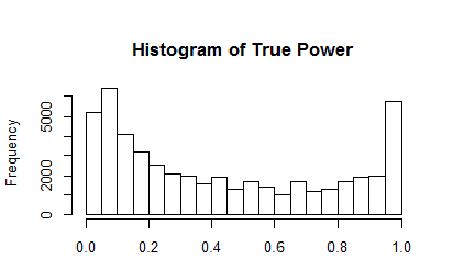
The histogram shows the distribution of true power across the 5,000 populations of studies.
The histogram shows that the simulation covers the full range of power. It also shows that high-powered studies are overrepresented because moderate to large effect sizes can achieve high power for a wide range of sample sizes. The distribution is not important for the evaluation of different estimation methods and benefits all estimation methods equally because observed power is a good estimator of true power when true power is close to the maximum (Yuan & Maxwell, 2005).
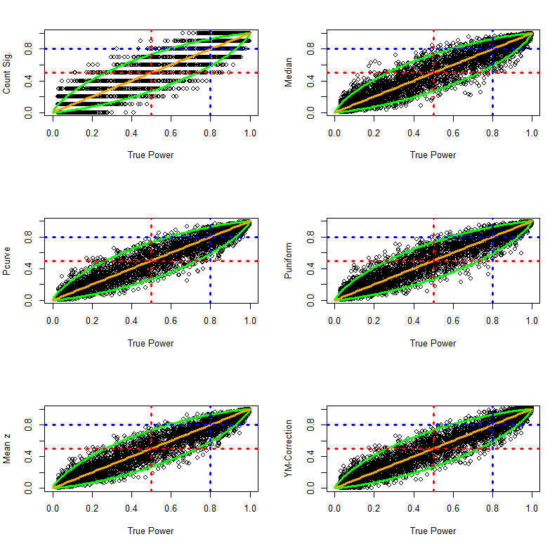
The next figure shows scatterplots of observed power as a function of true power. Values above the diagonal indicate that observed power overestimates true power. Values below the diagonal show that observed power underestimates true power.
Visual inspection of the plots suggests that all methods provide unbiased estimates of true power. Another observation is that the count of significant results provides the least accurate estimates of true power. The reason is simply that aggregation of dichotomous variables requires a large number of observations to approximate true power. The third observation is that visual inspection provides little information about the relative accuracy of the other methods. Finally, the plots show how accurate observed power estimates are in meta-analysis of 10 studies. When true power is 50%, estimates very rarely exceed 80%. Similarly, when true power is above 80%, observed power is never below 50%. Thus, observed power can be used to examine whether a set of studies met Cohen’s recommended guidelines to conduct studies with a minimum of 80% power. If observed power is 50%, it is nearly certain that the studies did not have the recommended 80% power.
To examine the relative accuracy of different estimation methods quantitatively, I computed bias scores (observed power – true power). As bias can overestimate and underestimate true power, the standard deviation of these bias scores can be used to quantify the precision of various estimation methods. In addition, I present the mean to examine whether a method has large sample accuracy (i.e. the bias approaches zero as the number of simulations increases). I also present the percentage of studies with no more than 20% points bias. Although 20% bias may seem large, it is not important to estimate power with very high precision. When observed power is below 50%, it suggests that a set of studies was underpowered even if the observed power estimate is an underestimation.
The quantitative analysis also shows no meaningful differences among the estimation methods. The more interesting question is how these methods perform under more challenging conditions when the set of studies are no longer exact replication studies with fixed power.
The next simulation simulated variation in sample sizes. For each population of studies, sample sizes were varied by multiplying a particular sample size by factors of 1 to 5.5 (1.0, 1.5,2.0…,5.5). Thus, a base-sample-size of 40 created a range of sample sizes from 40 to 220. A base-sample size of 100 created a range of sample sizes from 100 to 2,200. As variation in sample sizes increases the average sample size, the range of effect sizes was limited to a range from .004 to .4 and effect sizes were increased in steps of d = .004. The histogram shows the distribution of power in the 5,000 population of studies.
The simulation covers the full range of true power, although studies with low and very high power are overrepresented.
The results are visually not distinguishable from those in the previous simulation.
The quantitative comparison of the estimation methods also shows very similar results.
In sum, all methods perform well even when true power varies as a function of variation in sample sizes. This conclusion may not generalize to more extreme simulations of variation in sample sizes, but more extreme variations in sample sizes would further increase the average power of a set of studies because the average sample size would increase as well. Thus, variation in effect sizes poses a more realistic challenge for the different estimation methods.
Heterogeneous, Normally Distributed Effect Sizes
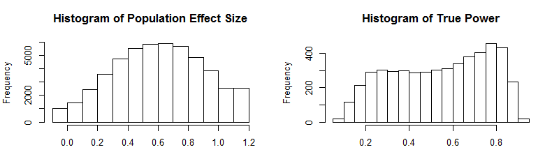
The next simulation used a random normal distribution of true effect sizes. Effect sizes were simulated to have a reasonable but large variation. Starting effect sizes ranged from .208 to 1.000 and increased in increments of .008. Sample sizes ranged from 10 to 60 and increased in increments of 2 to create 5,000 populations of studies. For each population of studies, effect sizes were sampled randomly from a normal distribution with a standard deviation of SD = .2. Extreme effect sizes below d = -.05 were set to -.05 and extreme effect sizes above d = 1.20 were set to 1.20. The first histogram of effect sizes shows the 50,000 population effect sizes. The histogram on the right shows the distribution of true power for the 5,000 sets of 10 studies.
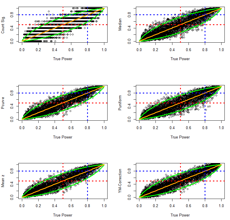
The plots of observed and true power show that the estimation methods continue to perform rather well even when population effect sizes are heterogeneous and normally distributed.
The quantitative comparison suggests that puniform has some problems with heterogeneity. More detailed studies are needed to examine whether this is a persistent problem for puniform, but given the good performance of the other methods it seems easier to use these methods.
Heterogeneous, Skewed Normal Effect Sizes
The next simulation puts the estimation methods to a stronger challenge by introducing skewed distributions of population effect sizes. For example, a set of studies may contain mostly small to moderate effect sizes, but a few studies examined large effect sizes. To simulated skewed effect size distributions, I used the rsnorm function of the fGarch package. The function creates a random distribution with a specified mean, standard deviation, and skew. I set the mean to d = .2, the standard deviation to SD = .2, and skew to 2. The histograms show the distribution of effect sizes and the distribution of true power for the 5,000 sets of studies (k = 10).
This time the results show differences between estimation methods in the ability of various estimation methods to deal with skewed heterogeneity. The percentage of significant results is unbiased, but is imprecise due to the problem of averaging dichotomous variables. The other methods show systematic deviations from the 95% confidence interval around the true parameter. Visual inspection suggests that the Yuan-Maxwell correction method has the best fit.
This impression is confirmed in quantitative analyses of bias. The quantitative comparison confirms major problems with the puniform estimation method. It also shows that the median, p-curve, and the average z-score method have the same slight positive bias. Only the Yuan-Maxwell corrected average power shows little systematic bias.
To examine biases in more detail, the following graphs plot bias as a function of true power. These plots can reveal that a method may have little average bias, but has different types of bias for different levels of power. The results show little evidence of systematic bias for the Yuan-Maxwell corrected average of power.
The following analyses examined bias separately for simulation with less or more than 50% true power. The results confirm that all methods except the Yuan-Maxwell correction underestimate power when true power is below 50%. In contrast, most estimation methods overestimate true power when true power is above 50%. The exception is puniform which still underestimated true power. More research needs to be done to understand the strange performance of puniform in this simulation. However, even if p-uniform could perform better, it is likely to be biased with skewed distributions of effect sizes because it assumes a fixed population effect size.
Conclusion
This investigation introduced and compared different methods to estimate true power for a set of studies. All estimation methods performed well when a set of studies had the same true power (exact replication studies), when effect sizes were homogenous and sample sizes varied, and when effect sizes were normally distributed and sample sizes were fixed. However, most estimation methods were systematically biased when the distribution of effect sizes was skewed. In this situation, most methods run into problems because the percentage of significant results is a function of the power of individual studies rather than the average power.
The results of these analyses suggest that the R-Index (Schimmack, 2014) can be improved by simply averaging power and then applying the Yuan-Maxwell correction. However, it is important to realize that the median method tends to overestimate power when power is greater than 50%. This makes it even more difficult for the R-Index to produce an estimate of low power when power is actually high. The next step in the investigation of observed power is to examine how different methods perform in unrepresentative (biased) sets of studies. In this case, the percentage of significant results is highly misleading. For example, Sterling et al. (1995) found percentages of 95% power, which would suggest that studies had 95% power. However, publication bias and questionable research practices create a bias in the sample of studies that are being published in journals. The question is whether other observed power estimates can reveal bias and can produce accurate estimates of the true power in a set of studies.