“What I’d like to say is that it is OK to criticize a paper, even [if, typo in original] it isn’t horrible.” (Gelman, 2023)
In this spirit, I would like to criticize Loken and Gelman’s confusing article about the interpretation of effect sizes in studies with small samples and selection for significance. They compare random measurement error to a backpack and the outcome of a study to running speed. Common sense suggests that the same individual under identical conditions would run faster without a backpack than with a backpack. The same outcome is also suggested by psychometric theories that suggest random measurement error attenuates population effect sizes, which would make it harder to demonstrate significance and produce, on average, weaker effect sizes.
The key point of Loken and Gelman’s article is to suggest that this intuition fails under some conditions. “Should we assume that if statistical significance is achieved in the presence of measurement error, the associated effects would have been stronger without noise? We caution against the fallacy”
To support their clam that common sense is a fallacy under certain conditions, they present the results of a simple simulation study. After some concerns about their conclusions were raised, Loken and Gelman shared the actual code of their simulation study. In this blog post, I share the code with annotations and reproduce their results. I also show that their results are based on selecting for significance only for the measure with random measurement error (with a backpack) and not for the measure without a backpack (no random measurement error). Reversing the selection shows that selection for significance without measurement error produces stronger effect sizes even more often than selection for significance with a backpack. Thus, it is not a fallacy to assume that we would all run faster without a backpack holding all other factors equal. However, a runner with a heavy backpack and tailwinds might run faster than a runner without a backpack facing strong headwinds. While this is true, the influence of wind on performance makes it difficult to see the influence of the backpack. Under identical conditions backpacks slow people down and random measurement error attenuates effects.
Loken and Gelman’s presentation of the results may explain why some readers, including us, misinterpreted their results to imply that selection bias and random measurement error may interaction in some complex way to produce even more inflated estimates of the true correlation. We added some lines of code to their simulation to compute the average correlations after selection for significance separately for the measure without error and the measure with error. This way, both measures benefit equally from selection bias. The plot also provides more direct evidence about the amount of bias that is introduced by selection bias and random measurement error. In addition, the plot shows the average 95% confidence intervals around the estimated correlation coefficients.
The plot shows that for large samples (N > 1,000), the measure without error always produces the expected true correlation of r = .15, whereas the measure with error always produces the expected attenuated correlation of r = .15 * .80 = .12. As sample sizes get smaller, the effect of selection bias becomes apparent. For the measure without error, the observed effect sizes are now inflated. For the measure with error, selection bias corrects for the inflation and the two biases cancel each other out to produce more accurate estimates of the true effect size than with the measure without error. For sample sizes below N = 400, however, both measures produce inflated estimates and in really small samples the attenuation effect due to unreliability is overwhelmed by selection bias. However, while the difference due to unreliability is negligible and approaches zero, it is clear that random measurement error combined with selection bias never produces even stronger estimates than the measure without error. Thus, it remains true that we should expect a measure without random measurement error to produce stronger correlations than a measure with random error. This fundamental principle of psychometrics, however, does not warrant the conclusion that an observed statistically significant correlation in small samples underestimates the true correlation coefficient because the correlation may have been inflated by selection for significance.
The plot also shows how researchers can avoid misinterpretation of inflated effect size estimates in small samples. In small samples, confidence intervals are wide. Figure 2 shows that the confidence interval around inflated effect size estimates in small samples is so wide that it includes the true correlation of r = .15. The width of the confidence interval in small samples make it clear that the study provided no meaningful information about the size of an effect. This does not mean the results are useless. After all, the results correctly show that the relationship between the variables is positive rather than negative. For the purpose of effect size estimation it is necessary to conduct meta-analysis and to include studies with significant and non-significant results. Furthermore, meta-analysis need to test for the presence of selection bias and correct for it when it is present.
P.S. If somebody claims that they ran a marathon in 2 hours with a heavy backpack, they may not be lying. They may just not tell you all of the information. We often fill in the blanks and that is where things can go wrong. If the backpack were a jet pack and the person was using it to fly for some of the race, we would no longer be surprised by the amazing feat. Similarly, if somebody tells you that they got a correlation of r = .8 in a sample of N = 8 with a measure that has only 20% reliable variance, you should not be surprised if they tell you that they got this result after picking 1 out of 20 studies because selection for significance will produce strong correlations in small samples even if there is no correlation at all. Once they tell you that they tried many times to get the one significant result, it is obvious that the next study is unlikely to replicate a significant result.
Sometimes You Can Be Faster With a Heavy Backpack
Annotated Original Code
### This is the final code used for the simulation studies posted by Andrew Gelman on his blog
### Comments are highlighted with my initials #US#
# First just the original two plots, high power N = 3000, low power N = 50, true slope = .15
r <- .15
sims<-array(0,c(1000,4))
xerror <- 0.5
yerror<-0.5
for (i in 1:1000) {
x <- rnorm(50,0,1)
y <- r*x + rnorm(50,0,1)
#US# this is a sloppy way to simulate a correlation of r = .15
#US# The proper code is r*x + rnorm(50,0,1)*sqrt(1-r^2)
#US# However, with the specific value of r = .15, the difference is trivial
#US# However, however, it raises some concerns about expertise
xx<-lm(y~x)
sims[i,1]<-summary(xx)$coefficients[2,1]
x<-x + rnorm(50,0,xerror)
y<-y + rnorm(50,0,yerror)
xx<-lm(y~x)
sims[i,2]<-summary(xx)$coefficients[2,1]
x <- rnorm(3000,0,1)
y <- r*x + rnorm(3000,0,1)
xx<-lm(y~x)
sims[i,3]<-summary(xx)$coefficients[2,1]
x<-x + rnorm(3000,0,xerror)
y<-y + rnorm(3000,0,yerror)
xx<-lm(y~x)
sims[i,4]<-summary(xx)$coefficients[2,1]
}
plot(sims[,2] ~ sims[,1],ylab=”Observed with added error”,xlab=”Ideal Study”)
abline(0,1,col=”red”)
plot(sims[,4] ~ sims[,3],ylab=”Observed with added error”,xlab=”Ideal Study”)
abline(0,1,col=”red”)
#US# There is no major issue with graphs 1 and 2.
#US# They merely show that high sampling error produces large uncertainty in the estimates.
#US# The small attenuation effect of r = .15 vs. r = 12 is overwhelmed by sampling error
#US# The real issue is the simulation of selection for significance in the third graph
# third graph
# run 2000 regressions at points between N = 50 and N = 3050
r <- .15
propor <-numeric(31)
powers<-seq(50,3050,100)
#US# These lines of code are added to illustrate the biased selection for significane
propor.reversed.selection <-numeric(31)
mean.sig.cor.without.error <- numeric(31) # mean correlation for the measure without error when t > 2
mean.sig.cor.with.error <- numeric(31) # mean correlation for the measure with error when t > 2
#US# It is sloppy to refer to sample sizes as powers.
#US# In between subject studies, the power to produce a true positive result
#US# is a function of the population correlation and the sample size
#US# With population correlations fixed at r = .15 or r = .12, sample size is the
#US# only variable that influences power
#US# However, power varies from alpha to 1 and it would be interesting to compare the
#US# power of studies with r = .15 and r = .12 to produce a significant result.
#US# The claim that “one would always run faster without a backback”
#US# could be interpreted as a claim that it is always easier to obtain a
#US# significant result without measurement error, r = .15, than with measurement error, r = .12
#US# This claim can be tested with Loken and Gelman’s simulation by computing
#US# the percentage of significant results obtained without and with measurement error
#US# Loken and Golman do not show this comparison of power.
#US# The reason might be the confusion of sample size with power.
#US# While sample sizes are held constant, power varies as a function of the population correlations
#US# without, r = .15, and with, r = .12, measurement error.
xerror<-0.5
yerror<-0.5
j = 1
i = 1
for (j in 1:31) {
sims<-array(0,c(1000,4))
for (i in 1:1000) {
x <- rnorm(powers[j],0,1)
y <- r*x + rnorm(powers[j],0,1)
#US# the same sloppy simulation of population correlations as before
xx<-lm(y~x)
sims[i,1:2]<-summary(xx)$coefficients[2,1:2]
x<-x + rnorm(powers[j],0,xerror)
y<-y + rnorm(powers[j],0,yerror)
xx<-lm(y~x)
sims[i,3:4]<-summary(xx)$coefficients[2,1:2]
}
#US# The code is the same as before, it just adds variation in sample sizes
#US# The crucial aspect to understand figure 3 is the following code that
#US# compares the results for the paired outcomes without and with measurement error
#US# Carlos Ungil (https://ch.linkedin.com/in/ungil) pointed out on Gelman’s blog #US# that there is another sloppy mistake in the simulation code that does not alter the results #US# The code compares absolute t-values (coefficient/sampling error), while the article #US# talks about inflated effect size estimates. However, while the sampling error variation #US# creates some variability, the pattern remains the same. #US# For sake of reproducibility I kept the comparison of t-values.
# find significant observations (t test > 2) and then check proportion
temp<-sims[abs(sims[,3]/sims[,4])> 2,]
#US# the use of t > 2 is sloppy and unnecessary.
#US# summary(lm) gives the exact p-values that could be used to select for significance
#US# summary(xx)[2,4] < .05
#US# However, this does not make a substantial difference
#US# The crucial part of this code is that it uses the outcomes of the simulation
#US# with random measurement error to select for significance
#US# As outcomes are paired, this means that the code sometimes selects outcomes
#US# in which sampling error produces significance with random measurement error
The z-curve analysis of results in this journal shows (a) that many published results are based on studies with low to modest power, (b) selection for significance inflates effect size estimates and the discovery rate of reported results, and (c) there is no evidence that research practices have changed over the past decade. Readers should be careful when they interpret results and recognize that reported effect sizes are likely to overestimate real effect sizes, and that replication studies with the same sample size may fail to produce a significant result again. To avoid misleading inferences, I suggest using alpha = .005 as a criterion for valid rejections of the null-hypothesis. Using this criterion, the risk of a false positive result is below 2%. I also recommend computing a 99% confidence interval rather than the traditional 95% confidence interval for the interpretation of effect size estimates.
Given the low power of many studies, readers also need to avoid the fallacy to report non-significant results as evidence for the absence of an effect. With 50% power, the results can easily switch in a replication study so that a significant result becomes non-significant and a non-significant result becomes significant. However, selection for significance will make it more likely that significant results become non-significant than observing a change in the opposite direction.
The average power of studies in a heterogeneous journal like Frontiers of Psychology provides only circumstantial evidence for the evaluation of results. When other information is available (e.g., z-curve analysis of a discipline, author, or topic, it may be more appropriate to use this information).
Report
Frontiers of Psychology was created in 2010 as a new online-only journal for psychology. It covers many different areas of psychology, although some areas have specialized Frontiers journals like Frontiers in Behavioral Neuroscience.
The business model of Frontiers journals relies on publishing fees of authors, while published articles are freely available to readers.
The number of articles in Frontiers of Psychology has increased quickly from 131 articles in 2010 to 8,072 articles in 2022 (source Web of Science). With over 8,000 published articles Frontiers of Psychology is an important outlet for psychological researchers to publish their work. Many specialized, print-journals publish fewer than 100 articles a year. Thus, Frontiers of Psychology offers a broad and large sample of psychological research that is equivalent to a composite of 80 or more specialized journals.
Another advantage of Frontiers of Psychology is that it has a relatively low rejection rate compared to specialized journals that have limited journal space. While high rejection rates may allow journals to prioritize exceptionally good research, articles published in Frontiers of Psychology are more likely to reflect the common research practices of psychologists.
To examine the replicability of research published in Frontiers of Psychology, I downloaded all published articles as PDF files, converted PDF files to text files, and extracted test-statistics (F, t, and z-tests) from published articles. Although this method does not capture all published results, there is no a priori reason that results reported in this format differ from other results. More importantly, changes in research practices such as higher power due to larger samples would be reflected in all statistical tests.
As Frontiers of Psychology only started shortly before the replication crisis in psychology increased awareness about the problem of low statistical power and selection for significance (publication bias), I was not able to examine replicability before 2011. I also found little evidence of changes in the years from 2010 to 2015. Therefore, I use this time period as the starting point and benchmark for future years.
Figure 1 shows a z-curve plot of results published from 2010 to 2014. All test-statistics are converted into z-scores. Z-scores greater than 1.96 (the solid red line) are statistically significant at alpha = .05 (two-sided) and typically used to claim a discovery (rejection of the null-hypothesis). Sometimes even z-scores between 1.65 (the dotted red line) and 1.96 are used to reject the null-hypothesis either as a one-sided test or as marginal significance. Using alpha = .05, the plot shows 71% significant results, which is called the observed discovery rate (ODR).
Visual inspection of the plot shows a peak of the distribution right at the significance criterion. It also shows that z-scores drop sharply on the left side of the peak when the results do not reach the criterion for significance. This wonky distribution cannot be explained with sampling error. Rather it shows a selective bias to publish significant results by means of questionable practices such as not reporting failed replication studies or inflating effect sizes by means of statistical tricks. To quantify the amount of selection bias, z-curve fits a model to the distribution of significant results and estimates the distribution of non-significant (i.e., the grey curve in the range of non-significant results). The discrepancy between the observed distribution and the expected distribution shows the file-drawer of missing non-significant results. Z-curve estimates that the reported significant results are only 31% of the estimated distribution. This is called the expected discovery rate (EDR). Thus, there are more than twice as many significant results as the statistical power of studies justifies (71% vs. 31%). Confidence intervals around these estimates show that the discrepancy is not just due to chance, but active selection for significance.
Using a formula developed by Soric (1989), it is possible to estimate the false discovery risk (FDR). That is, the probability that a significant result was obtained without a real effect (a type-I error). The estimated FDR is 12%. This may not be alarming, but the risk varies as a function of the strength of evidence (the magnitude of the z-score). Z-scores that correspond to p-values close to p =.05 have a higher false positive risk and large z-scores have a smaller false positive risk. Moreover, even true results are unlikely to replicate when significance was obtained with inflated effect sizes. The most optimistic estimate of replicability is the expected replication rate (ERR) of 69%. This estimate, however, assumes that a study can be replicated exactly, including the same sample size. Actual replication rates are often lower than the ERR and tend to fall between the EDR and ERR. Thus, the predicted replication rate is around 50%. This is slightly higher than the replication rate in the Open Science Collaboration replication of 100 studies which was 37%.
Figure 2 examines how things have changed in the next five years.
The observed discovery rate decreased slightly, but statistically significantly, from 71% to 66%. This shows that researchers reported more non-significant results. The expected discovery rate increased from 31% to 40%, but the overlapping confidence intervals imply that this is not a statistically significant increase at the alpha = .01 level. (if two 95%CI do not overlap, the difference is significant at around alpha = .01). Although smaller, the difference between the ODR of 60% and the EDR of 40% is statistically significant and shows that selection for significance continues. The ERR estimate did not change, indicating that significant results are not obtained with more power. Overall, these results show only modest improvements, suggesting that most researchers who publish in Frontiers in Psychology continue to conduct research in the same way as they did before, despite ample discussions about the need for methodological reforms such as a priori power analysis and reporting of non-significant results.
The results for 2020 show that the increase in the EDR was a statistical fluke rather than a trend. The EDR returned to the level of 2010-2015 (29% vs. 31), but the ODR remained lower than in the beginning, showing slightly more reporting of non-significant results. The size of the file drawer remains large with an ODR of 66% and an EDR of 72%.
The EDR results for 2021 look again better, but the difference to 2020 is not statistically significant. Moreover, the results in 2022 show a lower EDR that matches the EDR in the beginning.
Overall, these results show that results published in Frontiers in Psychology are selected for significance. While the observed discovery rate is in the upper 60%s, the expected discovery rate is around 35%. Thus, the ODR is nearly twice the rate of the power of studies to produce these results. Most concerning is that a decade of meta-psychological discussions about research practices has not produced any notable changes in the amount of selection bias or the power of studies to produce replicable results.
How should readers of Frontiers in Psychology articles deal with this evidence that some published results were obtained with low power and inflated effect sizes that will not replicate? One solution is to retrospectively change the significance criterion. Comparisons of the evidence in original studies and replication outcomes suggest that studies with a p-value below .005 tend to replicate at a rate of 80%, whereas studies with just significant p-values (.050 to .005) replicate at a much lower rate (Schimmack, 2022). Demanding stronger evidence also reduces the false positive risk. This is illustrated in the last figure that uses results from all years, given the lack of any time trend.
In the Figure the red solid line moved to z = 2.8; the value that corresponds to p = .005, two-sided. Using this more stringent criterion for significance, only 45% of the z-scores are significant. Another 25% were significant with alpha = .05, but are no longer significant with alpha = .005. As power decreases when alpha is set to more stringent, lower, levels, the EDR is also reduced to only 21%. Thus, there is still selection for significance. However, the more effective significance filter also selects for more studies with high power and the ERR remains at 72%, even with alpha = .005 for the replication study. If the replication study used the traditional alpha level of .05, the ERR would be even higher, which explains the finding that the actual replication rate for studies with p < .005 is about 80%.
The lower alpha also reduces the risk of false positive results, even though the EDR is reduced. The FDR is only 2%. Thus, the null-hypothesis is unlikely to be true. The caveat is that the standard null-hypothesis in psychology is the nil-hypothesis and that the population effect size might be too small to be of practical significance. Thus, readers who interpret results with p-values below .005 should also evaluate the confidence interval around the reported effect size, using the more conservative 99% confidence interval that correspondence to alpha = .005 rather than the traditional 95% confidence interval. In many cases, this confidence interval is likely to be wide and provide insufficient information about the strength of an effect.
Since 2011, it is an open secret that many published results in psychology journals do not replicate. The replicability of published results is particularly low in social psychology (Open Science Collaboration, 2015).
A key reason for low replicability is that researchers are rewarded for publishing as many articles as possible without concerns about the replicability of the published findings. This incentive structure is maintained by journal editors, review panels of granting agencies, and hiring and promotion committees at universities.
To change the incentive structure, I developed the Replicability Index, a blog that critically examined the replicability, credibility, and integrity of psychological science. In 2016, I created the first replicability rankings of psychology departments (Schimmack, 2016). Based on scientific criticisms of these methods, I have improved the selection process of articles to be used in departmental reviews.
1. I am using Web of Science to obtain lists of published articles from individual authors (Schimmack, 2022). This method minimizes the chance that articles that do not belong to an author are included in a replicability analysis. It also allows me to classify researchers into areas based on the frequency of publications in specialized journals. Currently, I cannot evaluate neuroscience research. So, the rankings are limited to cognitive, social, developmental, clinical, and applied psychologists.
2. I am using department’s websites to identify researchers that belong to the psychology department. This eliminates articles that are from other departments.
3. I am only using tenured, active professors. This eliminates emeritus professors from the evaluation of departments. I am not including assistant professors because the published results might negatively impact their chances to get tenure. Another reason is that they often do not have enough publications at their current university to produce meaningful results.
Like all empirical research, the present results rely on a number of assumptions and have some limitations. The main limitations are that (a) only results that were found in an automatic search are included (b) only results published in 120 journals are included (see list of journals) (c) published significant results (p < .05) may not be a representative sample of all significant results (d) point estimates are imprecise and can vary based on sampling error alone.
These limitations do not invalidate the results. Large difference in replicability estimates are likely to predict real differences in success rates of actual replication studies (Schimmack, 2022).
New York University
I used the department website to find core members of the psychology department. I found 13 professors and 6 associate professors. Figure 1 shows the z-curve for all 12,365 tests statistics in articles published by these 19 faculty members. I use the Figure to explain how a z-curve analysis provides information about replicability and other useful meta-statistics.
1. All test-statistics are converted into absolute z-scores as a common metric of the strength of evidence (effect size over sampling error) against the null-hypothesis (typically H0 = no effect). A z-curve plot is a histogram of absolute z-scores in the range from 0 to 6. The 1,239 (~ 10%) of z-scores greater than 6 are not shown because z-scores of this magnitude are extremely unlikely to occur when the null-hypothesis is true (particle physics uses z > 5 for significance). Although they are not shown, they are included in the meta-statistics.
2. Visual inspection of the histogram shows a steep drop in frequencies at z = 1.96 (dashed blue/red line) that corresponds to the standard criterion for statistical significance, p = .05 (two-tailed). This shows that published results are selected for significance. The dashed red/white line shows significance for p < .10, which is often used for marginal significance. There is another drop around this level of significance.
3. To quantify the amount of selection bias, z-curve fits a statistical model to the distribution of statistically significant results (z > 1.96). The grey curve shows the predicted values for the observed significant results and the unobserved non-significant results. The full grey curve is not shown to present a clear picture of the observed distribution. The statistically significant results (including z > 6) make up 20% of the total area under the grey curve. This is called the expected discovery rate because the results provide an estimate of the percentage of significant results that researchers actually obtain in their statistical analyses. In comparison, the percentage of significant results (including z > 6) includes 70% of the published results. This percentage is called the observed discovery rate, which is the rate of significant results in published journal articles. The difference between a 70% ODR and a 20% EDR provides an estimate of the extent of selection for significance. The difference of 50 percentage points is large. The upper level of the 95% confidence interval for the EDR is 28%. Thus, the discrepancy is not just random. To put this result in context, it is possible to compare it to the average for 120 psychology journals in 2010 (Schimmack, 2022). The ODR is similar (70 vs. 72%), but the EDR is a bit lower (20% vs. 28%), although the difference might be largely due to chance.
4. The EDR can be used to estimate the risk that published results are false positives (i.e., a statistically significant result when H0 is true), using Soric’s (1989) formula for the maximum false discovery rate. An EDR of 20% implies that no more than 20% of the significant results are false positives, however the upper limit of the 95%CI of the EDR, 28%, allows for 36% false positive results. Most readers are likely to agree that this is an unacceptably high risk that published results are false positives. One solution to this problem is to lower the conventional criterion for statistical significance (Benjamin et al., 2017). Figure 2 shows that alpha = .005 reduces the point estimate of the FDR to 3% with an upper limit of the 95% confidence interval of XX%. Thus, without any further information readers could use this criterion to interpret results published by NYU faculty members.
5. The estimated replication rate is based on the mean power of significant studies (Brunner & Schimmack, 2020). Under ideal condition, mean power is a predictor of the success rate in exact replication studies with the same sample sizes as the original studies. However, as NYU professor van Bavel pointed out in an article, replication studies are never exact, especially in social psychology (van Bavel et al., 2016). This implies that actual replication studies have a lower probability of producing a significant result, especially if selection for significance is large. In the worst case scenario, replication studies are not more powerful than original studies before selection for significance. Thus, the EDR provides an estimate of the worst possible success rate in actual replication studies. In the absence of further information, I have proposed to use the average of the EDR and ERR as a predictor of actual replication outcomes. With an ERR of 62% and an EDR of 20%, this implies an actual replication prediction of 41%. This is close to the actual replication rate in the Open Science Reproducibility Project (Open Science Collaboration, 2015). The prediction for results published in 120 journals in 2010 was (ERR = 67% + ERR = 28%)/ 2 = 48%. This suggests that results published by NYU faculty are slightly less replicable than the average result published in psychology journals, but the difference is relatively small and might be mostly due to chance.
6. There are two reasons for low replication rates in psychology. One possibility is that psychologists test many false hypotheses (i.e., H0 is true) and many false positive results are published. False positive results have a very low chance of replicating in actual replication studies (i.e. 5% when .05 is used to reject H0), and will lower the rate of actual replications a lot. Alternative, it is possible that psychologists tests true hypotheses (H0 is false), but with low statistical power (Cohen, 1961). It is difficult to distinguish between these two explanations because the actual rate of false positive results is unknown. However, it is possible to estimate the typical power of true hypotheses tests using Soric’s FDR. If 20% of the significant results are false positives, the power of the 80% true positives has to be (.62 – .2*.05)/.8 = 76%. This would be close to Cohen’s recommended level of 80%, but with a high level of false positive results. Alternatively, the null-hypothesis may never be really true. In this case, the ERR is an estimate of the average power to get a significant result for a true hypothesis. Thus, power is estimated to be between 62% and 76%. The main problem is that this is an average and that many studies have less power. This can be seen in Figure 1 by examining the local power estimates for different levels of z-scores. For z-scores between 2 and 2.5, the ERR is only 47%. Thus, many studies are underpowered and have a low probability of a successful replication with the same sample size even if they showed a true effect.
Area
The results in Figure 1 provide highly aggregated information about replicability of research published by NYU faculty. The following analyses examine potential moderators. First, I examined social and cognitive research. Other areas were too small to be analyzed individually.
The z-curve for the 11 social psychologists was similar to the z-curve in Figure 1 because they provided more test statistics and had a stronger influence on the overall result.
The z-curve for the 6 cognitive psychologists looks different. The EDR and ERR are higher for cognitive psychology, and the 95%CI for social and cognitive psychology do not overlap. This suggests systematic differences between the two fields. These results are consistent with other comparisons of the two fields, including actual replication outcomes (OSC, 2015). With an EDR of 44%, the false discovery risk for cognitive psychology is only 7% with an upper limit of the 95%CI at 12%. This suggests that the conventional criterion of .05 does keep the false positive risk at a reasonably low level or that an adjustment to alpha = .01 is sufficient. In sum, the results show that results published by cognitive researchers at NYU are more replicable than those published by social psychologists.
Position
Since 2015 research practices in some areas of psychology, especially social psychology, have changed to increase replicability. This would imply that research by younger researchers is more replicable than research by more senior researchers that have more publications before 2015. A generation effect would also imply that a department’s replicability increases when older faculty members retire. On the other hand, associate professors are relatively young and likely to influence the reputation of a department for a long time.
The figure above shows that most test statistics come from the (k = 13) professors. As a result, the z-curve looks similar to the z-curve for all test values in Figure 1. The results for the 6 associate professors (below) are more interesting. Although five of the six associate professors are in the social area, the z-curve results show a higher EDR and less selection bias than the plot for all social psychologists. This suggests that the department will improve when full professors in social psychology retire.
Some researchers have changed research practices in response to the replication crisis. It is therefore interesting to examine whether replicability of newer research has improved. To examine this question, I performed a z-curve analysis for articles published in the past five year (2016-2021).
The results show very little signs of improvement. The EDR increased from 20% to 26%, but the confidence intervals are too wide to infer that this is a systematic change. In contrast, Stanford University improved from 22% to 50%, a significant increase. For now, NYU results should be interpreted with alpha = .005 as threshold for significance to maintain a reasonable false positive risk.
The table below shows the meta-statistics of all 19 faculty members. You can see the z-curve for each faculty member by clicking on their name.
Gordon et al. (2021) conducted a meta-analysis of 103 studies that were included in prediction markets to forecast the outcome of replication studies. The results show that prediction markets can forecast replication outcomes above chance levels, but the value of this information is limited. Without actual replication studies, it remains unclear which published results can be trusted or not. Here I compare the performance of prediction markets to the R-Index and the closely related p < .005 rule. These statistical forecasts perform nearly as well as markets and are much easier to use to make sense of thousands of published articles. However, even these methods have a high failure rate. The best solution to this problem is to rely on meta-analyses of studies rather than to predict the outcome of a single study. In addition to meta-analyses, it will be necessary to conduct new studies that are conducted with high scientific integrity to provide solid empirical foundations for psychology. Claims that are not supported by bias-corrected meta-analyses or new preregistered studies are merely suggestive and currently lack empirical support.
Introduction
Since 2011, it became apparent that many published results in psychology, especially social psychology fail to replicate in direct replication studies (Open Science Collaboration, 2015). In social psychology the success rate of replication studies is so low (25%) that it makes sense to bet on replication failures. This would produce 75% successful outcomes, but it would also imply that an entire literature has to be discarded.
It is practically impossible to redo all of the published studies to assess their replicability. Thus, several projects have attempted to predict replication outcomes of individual studies. One strategy is to conduct prediction markets in which participants can earn real money by betting on replication outcomes. There have been four prediction markets with a total of 103 studies with known replication outcomes (Gordon et al., 2021). The key findings are summarized in Table 1.
Markets have a good overall success rate, (28+47)/103 = 73% that is above chance (flipping a coin). Prediction markets are better at predicting failures, 28/31 = 90%, than predicting successes, 47/72 = 65%. The modest success rate for success is a problem because it would be more valuable to be able to identify studies that will replicate and do not require a new study to verify the results.
Another strategy to predict replication outcomes relies on the fact that the p-values of original studies and the p-values of replication studies are influenced by the statistical power of a study (Brunner & Schimmack, 2020). Studies with higher power are more likely to produce lower p-values and more likely to produce significant p-values in replication studies. As a result, p-values also contain valuable information about replication outcomes. Gordon et al. (2021) used p < .005 as a rule to predict replication outcomes. Table 2 shows the performance of this simple rule.
The overall success rate of this rule is nearly as good as the prediction markets, (39+35)/103 = 72%; a difference by k = 1 studies. The rule does not predict failures as well as the markets, 39/54 = 72% (vs. 90%), but it predicts successes slightly better than the markets, 35/49 = 71% (vs. 65%).
A logistic regression analysis showed that both predictors independently contribute to the prediction of replication outcomes, market b = 2.50, se = .68, p = .0002; p < .005 rule: b = 1.44, se = .48, p = .003.
In short, p-values provide valuable information about the outcome of replication studies.
The R-Index
Although a correlation between p-values and replication outcomes follows logically from the influence of power on p-values in original and replication studies, the cut-off value of .005 appears to be arbitrary. Gordon et al. (2017) justify its choice with an article by Benjamin et al. (2017) that recommended a lower significance level (alpha) to ensure a lower false positive risk. Moreover, they advocated for this rule for new studies that preregister hypotheses and do not suffer from selection bias. In contrast, the replication crisis was caused by selection for significance which produced success rates of 90% or more in psychology journals (Motyl et al., 2017; Sterling, 1959; Sterling et al., 1995). One main reason for replication failures is that selection for significance inflates effect sizes and due to regression to the mean, effect sizes in replication studies are bound to be weaker, resulting in non-significant results, especially if the original p-value was close to the threshold value of alpha = .05. The Open Science Collaboration (2015) replicability project showed that effect sizes are on average inflated by over 100%.
The R-Index provides a theoretical rational for the choice of a cut-off value for p-values. The theoretical cutoff value happens to be p = .0084. The fact that it is close to Benjamin et al.’s (2017) value of .005 is merely a coincidence.
P-values can be transformed into estimates of the statistical power of a study. These estimates rely on the observed effect size of a study and are sometimes called observed power or post-hoc power because power is computed after the results of a study are known. Figure 1 illustrates observed power with an example of a z-test that produced a z-statistic of 2.8 which corresponds to a two-sided p-value of .005.
A p-value of .005 corresponds to z-value of 2.8 for the standard normal distribution centered over zero (the nil-hypothesis). The standard level of statistical significance, alpha = .05 (two-sided) corresponds to z-value of 1.96. Figure 1 shows the sampling distribution of studies with a non-central z-score of 2.8. The green line cuts this distribution into a smaller area of 20% below the significance level and a larger area of 80% above the significance level. Thus, the observed power is 80%.
Selection for significance implies truncating the normal distribution at the level of significance. This means the 20% of non-significant results are discarded. As a result, the median of the truncated distribution is higher than the median of the full normal distribution. The new median can be found using the truncnorm package in R.
qtruncnorm(.5,a = qnorm(1-.05/2),mean=2.8) = 3.05
This value corresponds to an observed power of
qnorm(3.05,qnorm(1-.05/2) = .86
Thus, selection for significance inflates observed power of 80% to 86%. The amount of inflation is larger when power is lower. With 20% power, the inflated power after selection for significance is 67%.
Figure 3 shows the relationship between inflated power on the x-axis and adjusted power on the y-axis. The blue curve uses the truncnorm package. The green line shows the simplified R-Index that simply substracts the amount of inflation from the inflated power. For example, if inflated power is 86%, the inflation is 1-.86 = 14% and subtracting the inflation gives an R-Index of 86-14 = 82%. This is close to the actual value of 80% that produced the inflated value of 86%.
Figure 4 shows that the R-Index is conservative (underestimates power) when power is over 50%, but is liberal (overestimates power) when power is below 50%. The two methods are identical when power is 50% and inflated power is 75%. This is a fortunate co-incidence because studies with more than 50% power are expected to replicate and studies with less than 50% power are expected to fail in a replication attempt. Thus, the simple R-Index makes the same dichotomous predictions about replication outcomes as the more sophisticated approach to find the median of the truncated normal distribution.
The inflated power for actual power of 50% is 75% and 75% power corresponds to a z-score of 2.63, which in turn corresponds to a p-value of p = .0084.
Performance of the R-Index is slightly worse than the p < .005 rule because the R-Index predicts 5 more successes, but 4 of these predictions are failures. Given the small sample size, it is not clear whether this difference is reliable.
In sum, the R-Index is based on a transformation of p-values into estimates of statistical power, while taking into account that observed power is inflated when studies are selected for significance. It provides a theoretical rational for the atheoretical p < .005 rule, because this rule roughly cuts p-values into p-values with more or less than 50% power.
Predicting Success Rates
The overall success rate across the 103 replication studies was 50/103 = 49%. This percentage cannot be generalized to a specific population of studies because the 103 are not a representative sample of studies. Only the Open Science Collaboration project used somewhat representative sampling. However, the 49% success rate can be compared to the success rates of different prediction methods. For example, prediction markets predict a success rate of 72/103 = 70%, a significant difference (Gordon et al., 2021). In contrast, the R-Index predicts a success rate of 54/103 = 52%, which is closer to the actual success rate. The p < .005 rule does even better with a predicted success rate of 49/103 = 48%.
Another method that has been developed to estimate the expected replication rate is z-curve (Bartos & Schimmack, 2021; Brunner & Schimmack, 2020). Z-curve transforms p-values into z-scores and then fits a finite mixture model to the distribution of significant p-values. Figure 5 illustrates z-curve with the p-values from the 103 replicated studies.
The z-curve estimate of the expected replication rate is 60%. This is better than the prediction market, but worse than the R-Index or the p < .005 rule. However, the 95%CI around the ERR includes the true value of 49%. Thus, sampling error alone might explain this discrepancy. However, Bartos and Schimmack (2021) discussed several other reasons why the ERR may overestimate the success rate of actual replication studies. One reason is that actual replication studies are not perfect replicas of the original studies. So called, hidden moderators may create differences between original and replication studies. In this case, selection for significance produces even more inflation that the model assumes. In the worst case scenario, a better estimate of actual replication outcomes might be the expected discovery rate (EDR), which is the power of all studies that were conducted, including non-significant studies. The EDR for the 103 studies is 28%, but the 95%CI is wide and includes the actual rate of 49%. Thus, the dataset is too small to decide between the ERR or the EDR as best estimates of actual replication outcomes. At present it is best to consider the EDR the worst possible and the ERR the best possible scenario and to expect the actual replication rate to fall within this interval.
Social Psychology
The 103 studies cover studies from experimental economics, cognitive psychology, and social psychology. Social psychology has the largest set of studies (k = 54) and the lowest success rate, 33%. The prediction markets overpredict successes, 50%. The R-Index also overpredicted successes, 46%. The p < .005 rule had the least amount of bias, 41%.
Z-curve predicted an ERR of 55% s and the actual success rate fell outside the 95% confidence interval, 34% to 74%. The EDR of 22% underestimates the success rate, but the 95%CI is wide and includes the true value, 95%CI = 5% to 70%. Once more the actual success rate is between the EDR and the ERR estimates, 22% < 34% < 55%.
In short, prediction models appear to overpredict replication outcomes in social psychology. One reason for this might be that hidden moderators make it difficult to replicate studies in social psychology which adds additional uncertainty to the outcome of replication studies.
Regarding predictions of individual studies, prediction markets achieved an overall success rate of 76%. Prediction markets were good at predicting failures, 25/27 = 93%, but not so good in predicting successes, 16/27 = 59%.
The R-Index performed as well as the prediction markets with one more prediction of a replication failure.
The p < .005 rule was the best predictor because it predicted more replication failures.
Performance could be increased by combining prediction markets and the R-Index and only bet on successes when both predictors predicted a success. In particular, the prediction of success improved to 14/19 = 74%. However, due to the small sample size it is not clear whether this is a reliable finding.
Non-Social Studies
The remaining k = 56 studies had a higher success rate, 65%. The prediction markets overpredicted success, 92%. The R-Index underpredicted successes, 59%. The p < .005 rule underpredicted successes even more.
This time z-curve made the best prediction with an ERR of 67%, 95%CI = 45% to 86%. The EDR underestimates the replication rate, although the 95%CI is very wide and includes the actual success rate, 5% to 81%. The fact that z-curve overestimated replicability for social psychology, but not for other areas, suggests that hidden moderators may contribute to the replication problems in social psychology.
For predictions of individual outcomes, prediction markets had a success rate of (3 + 31)/49 = 76%. The good performance is due to the high success rate. Simply betting on success would have produced 32/49 = 65% successes. Predictions of failures had a s success rate of 3/4 = 75% and predictions of successes had a success rate of 31/45 = 69%.
The R-Index had a lower success rate of (9 +21)/49 = 61%. The R-Index was particularly poor at predicting failures, 9/20 = 45%, but was slightly better at predicting successes than the prediction markets, 21/29 = 72%.
The p < .500 rule had a success rate equal to the R-Index, (10 + 20)/49 = 61%, with one more correctly predicted failure and one less correctly predicted success.
Discussion
The present results reproduce the key findings of Gordon et al. (2021). First, prediction markets overestimate the success of actual replication studies. Second, prediction markets have some predictive validity in forecasting the outcome of individual replication studies. Third, a simple rule based on p-values also can forecast replication outcomes.
The present results also extend Gordon et al.’s (2021) findings based on additional analyses. First, I compared the performance of prediction markets to z-curve as a method for the prediction of the success rates of replication outcomes (Bartos & Schimmack, 2021; Brunner & Schimmack, 2021). Z-curve overpredicted success rates for all studies and for social psychology, but was very accurate for the remaining studies (economics, cognition). In all three comparisons, z-curve performed better than prediction markets. Z-curve also has several additional advantages over prediction markets. First, it is much easier to code a large set of test statistics than to run prediction markets. As a result, z-curve has already been used to estimate the replication rates for social psychology based on thousands of test statistics, whereas estimates of prediction markets are based on just over 50 studies. Second, z-curve is based on sound statistical principles that link the outcomes of original studies to the outcomes of replication studies (Brunner & Schimmack, 2020). In contrast, prediction markets rest on unknown knowledge of market participants that can vary across markets. Third, z-curve estimates are provided with validated information about the uncertainty in the estimates, whereas prediction markets provide no information about uncertainty and uncertainty is large because markets tend to be small. In conclusion, z-curve is more efficient and provides better estimates of replication rates than prediction markets.
The main goal of prediction markets is to assess the credibility of individual studies. Ideally, prediction markets would help consumers of published research to distinguish between studies that produced real findings (true positives) and studies that produced false findings (false positives) without the need to run additional studies. The encouraging finding is that prediction markets have some predictive validity and can distinguish between studies that replicate and studies that do not replicate. However, to be practically useful it is necessary to assess the practical usefulness of the information that is provided by prediction markets. Here we need to distinguish the practical consequences of replication failures and successes. Within the statistical framework of nil-hypothesis significance testing, successes and failures have different consequences.
A replication failure increases uncertainty about the original finding. Thus, more research is needed to understand why the results diverged. This is also true for market predictions. Predictions that a study would fail to replicate cast doubt about the original study, but do not provide conclusive evidence that the original study reported a false positive result. Thus, further studies are needed, even if a market predicts a failure. In contrast, successes are more informative. Replicating a previous finding successfully strengthens the original findings and provides fairly strong evidence that a finding was not a false positive result. Unfortunately, the mere prediction that a finding will replicate does not provide the same reassurance because markets only have an accuracy of about 70% when they predict a successful replication. The p < .500 rule is much easier to implement, but its ability to forecast successes is also around 70%. Thus, neither markets nor a simple statistical rule are accurate enough to avoid actual replication studies.
Meta-Analysis
The main problem of prediction markets and other forecasting projects is that single studies are rarely enough to provide evidence that is strong enough to evaluate theoretical claims. It is therefore not particularly important whether one study can be replicated successfully or not, especially when direct replications are difficult or impossible. For this reason, psychologists have relied for a long time on meta-analyses of similar studies to evaluate theoretical claims.
It is surprising that prediction markets have forecasted the outcome of studies that have been replicated many times before the outcome of a new replication study was predicted. Take the replication of Schwarz, Strack, and Mai (1991) in Many Labs 2 as an example. This study manipulated the item-order of questions about marital satisfaction and life-satisfaction and suggested that a question about marital satisfaction can prime information that is used in life-satisfaction judgments. Schimmack and Oishi (2005) conducted a meta-analysis of the literature and showed that the results by Schwarz et al. (1991) were unusual and that the actual effect size is much smaller. Apparently, the market participants were unaware of this meta-analysis and predicted that the original result would replicate successfully (probability of success = 72%). Contrary to the market, the study failed to replicate. This example suggests that meta-analyses might be more valuable than prediction markets or the p-value of a single study.
The main obstacle for the use of meta-analyses is that many published meta-analyses fail to take selection for significance into account and overestimate replicability. However, new statistical methods that correct for selection bias may address this problem. The R-Index is a rather simple tool that allows to correct for selection bias in small sets of studies. I use the article by Nairne et al. (2008) that was used for the OSC project as an example. The replication project focused on Study 2 that produced a p-value of .026. Based on this weak evidence alone, the R-Index would predict a replication failure (observed power = .61, inflation = .39, R-Index = .61 – .39 = .22). However, Study 1 produced much more convincing evidence for the effect, p = .0007. If this study had been picked for the replication attempt, the R-Index would have predicted a successful outcome (observed power = .92, inflation = .08, R-Index = .84). A meta-analysis would average across the two power estimates and also predict a successful replication outcome (mean observed power = .77, inflation = .23, R-Index = .53). The actual replication study was significant with p = .007 (observed power = .77, inflation = .23, R-Index = .53). A meta-analysis across all three studies also suggests that the next study will be a successful replication (R-Index = .53), but the R-Index also shows that replication failures are likely because the studies have relatively low power. In short, prediction markets may be useful when only a single study is available, but meta-analysis are likely to be superior predictors of replication outcomes when prior replication studies are available.
Conclusion
Gordon et al. (2021) conducted a meta-analysis of 103 studies that were included in prediction markets to forecast the outcome of replication studies. The results show that prediction markets can forecast replication outcomes above chance levels, but the value of this information is limited. Without actual replication studies, it remains unclear which published results can be trusted or not. Statistical methods that simply focus on the strength of evidence in original studies perform nearly as well and are much easier to use to make sense of thousands of published articles. However, even these methods have a high failure rate. The best solution to this problem is to rely on meta-analyses of studies rather than to predict the outcome of a single study. In addition to meta-analyses, it will be necessary to conduct new studies that are conducted with high scientific integrity to provide solid empirical foundations for psychology.
I reinvestigate the performance of prediction markets for the Open Science Collaboration replicability project. I show that performance of prediction markets varied considerably across the two markets, with the second market failing to replicate the excellent performance of the first market. I also show that the markets did not perform significantly better than a “burn everything to the ground” rule that bets on failure every time. Finally, I suggest a simple rule that can be easily applied to published studies that only treats results with p-values below .005 as significant. Finally, I discuss betting on future studies as a way to optimize resource allocation for future studies.
Introduction
For decades, psychologists failed to properly test their hypotheses. Statistically significant results in journals are meaningless because published results are selected for significance. A replication project with 100 studies from three journals that reported significant results found that only 37% (36/97) of published significant results could be replicated (Open Science Collaboration, 2015).
Unfortunately, it is impossible to rely on actual replication studies to examine the credibility of thousands of findings that have been reported over the years. Dreber, Pfeiffer, Almenberg, Isakssona, Wilson, Chen, Nosek, and Johannesson (2015) proposed prediction markets as a solution to this problem. Prediction markets rely on a small number of traders to bet on the outcome of replication studies. They can earn a small amount of real money for betting on studies that actually replicate.
To examine the forecasting abilities of prediction markets, Dreber et al. (2015) conducted two studies. The first study with 23 studies started in November 2012 and lasted two month (N = 47 participants). The second study with 21 studies started in October 2014 (N = 45 participants). The studies are very similar to each other. Thus, we can consider Study 2 a close replication of Study 1.
Studies were selected from the set of 100 studies based on time of completion. To pay participants, studies were chosen that were scheduled to be completed within two month after the completion of the prediction market. It is unclear how completion time may influence the type of study that was included or the outcome of the included studies.
The published article reports the aggregated results across the two studies. A market price above 50% was considered to be a prediction of a successful replication and a market price below 50% was considered to be a prediction of a replication failure. The key finding was that “the prediction markets correctly predict the outcome of 71% of the replications (29 of 41 studies” (p. 15344). The authors compare this finding to a proverbial coin flip which implies a replication rate of 50% and find that 71% is [statistically] significantly higher than than 50%.
Below I am conducting some additional statistical analyses of the open data. First, we can compare the performance of the prediction market with a different prediction rule. Given the higher prevalence of replication failures than successes, a simple rule is to use the higher base rate of failures to predict that all studies will fail to replicate. As the failure rate for the total set of 97 studies was 37%, this prediction rule has a success rate of 1-.37 = 63%. For the 43 studies with significant results, the success rate of replication studies was also 37% (15/41). Somewhat surprisingly, the success rates were also close to 37% for Prediction Market 1, 32% (7/22) and Prediction Market 2, 42% (8 / 19).
In comparison to a simple prediction rule that everything in psychology journals does not replicate, prediction markets are no longer statistically significantly better, chi2(1) = 1.82, p = .177.
Closer inspection of the original data also revealed a notable difference in the performance of the two prediction markets. Table 1 shows the results separately for prediction markets 1 and 2. Whereas the performance of the first prediction market is nearly perfect, 91% (20/22), the replication market performed only at chance levels (flip a coin), 53% (10/19). Despite the small sample size, the success rates in the two studies are statistically significantly different, chi2(1) = 5.78, p = .016.
There is no explanation for these discrepancies and the average result reported in the article can still be considered the best estimate of prediction markets’ performance, but trust in their ability is diminished by the fact that a close replication of excellent performance failed to replicate. Not reporting the different outcomes for two separate studies could be considered a questionable decision.
The main appeal of prediction markets over the nihilistic trash-everything rule is that decades of research would have produced some successes. However, the disadvantage of prediction markets is that they take a long time, cost money, and the success rates are currently uncertain. A better solution might be to find rules that can be applied easily to large sets of studies (Yang, Wu, & Uzzi, 2020). One simple rule is suggested by the simple relationship between strength of evidence and replicability. The stronger the evidence against the null-hypothesis is (i.e., lower p-values), the more likely it is that the original study had high power and that the results will replicate in a replication study. There is no clear criterion for a cut-off point to optimize prediction, but the results of the replication project can be used to validate cut-off points empirically.
One suggests has been to consider only p-values below .005 as statistically significant (Benjamin et al., 2017). This rule is especially useful when selection bias is present. Selection bias can produce many results with p-values between .05 and .005 that have low power. However, p-values below .005 are more difficult to produce with statistical tricks.
The overall success rate for the 41 studies included in the Prediction Markets was 63% (26/41), a difference of 4 studies. The rule also did better for the first market, 81% (18.22) than for the second market, 42% (8/19).
Table 2 shows that the main difference between the two markets was that the first market contained more studies with questionable p-values between .05 and .005 (15 vs. 6). For the second market, the rule overpredicts successes and there are more false (8) than correct (5) predictions. This finding is consistent with examinations of the total set of replication studies in the replicability project (Schimmack, 2015). Based on this observation, I recommended a 4-sigma rule, p < .00006. The overall success rate increases to 68% (28/41) and improvement by 2 studies. However, an inspection of correct predictions of successes shows that the rule only correctly predicts 5 of the 15 successes (33%), whereas the p < .005 rule correctly predicted 10 of the 15 successes (67%). Thus, the p < .005 rule has the advantage that it salvages more studies.
Conclusion
Meta-scientists are still scientists and scientists are motivated to present their results in the best possible light. This is also true for Derber et al.’s (2015) article. The authors enthusiastically recommend prediction markets as a tool “to quickly identify findings that are unlikely to replicate” Based on their meta-analysis of two prediction markets with a total of just 41 studies, the authors conclude that “prediction markets are well suited” to assess the replicability of published results in psychology. I am not the only one to point out that this conclusion is exaggerated (Yang, Wu, & Uzzi, 2020). First, prediction markets are not quick at identifying replicable results, especially when we compare the method to a simple computation of the exact p-values to decide whether the p-value is below .005 or not. It is telling that nobody has used prediction markets to forecast the outcome of new replication studies. One problem is that a market requires a set of studies, which makes it difficult to use them to predict outcomes of single studies. It is also unclear how well prediction markets really work. The original article omitted the fact that it worked extremely well in the first market and not at all in the second market, a statistically significant difference. The outcome seems to depend a lot on the selection of studies in the market. Finally, I showed that a simple statistical rule alone can predict replication outcomes nearly as well as prediction markets.
There is no reason to use markets for multiple studies. One could also set up betting for individual studies, just like individuals can bet on the outcome of a single match in sports or a single election outcome. Betting might be more usefully employed for the prediction of original studies than to vet the outcome of replication studies. For example, if everybody bets that a study will produce a significant result, there appears to be little uncertainty about the outcome, and the actual study may be a waste of resources. One concerns in psychology is that many studies merely produce significant p-values for obvious predictions. Betting on effect sizes would help to make effect sizes more important. If everybody bets on a very small effect size a study might not be useful to run because the expected effect size is trivial, even if the effect is greater than zero. Betting on effect sizes could also be used for informal power analyses to determine the sample size of the actual study.
References
Dreber, A., Pfeiffer, T., Almenberg, J., Isaksson, S., Wilson, B., Chen, Y., Nosek, B. A., & Johannesson, M. (2015). Using prediction markets to estimate the reproducibility of scientific research. PNAS Proceedings of the National Academy of Sciences of the United States of America, 112(50), 15343–15347. https://doi.org/10.1073/pnas.1516179112 1 commen
Information about the replicability of published results is important because empirical results can only be used as evidence if the results can be replicated. However, the replicability of published results in social psychology is doubtful. Brunner and Schimmack (2020) developed a statistical method called z-curve to estimate how replicable a set of significant results are, if the studies were replicated exactly. In a replicability audit, I am applying z-curve to the most cited articles of psychologists to estimate the replicability of their studies.
John A. Bargh
Bargh is an eminent social psychologist (H-Index in WebofScience = 61). He is best known for his claim that unconscious processes have a strong influence on behavior. Some of his most cited article used subliminal or unobtrusive priming to provide evidence for this claim.
Bargh also played a significant role in the replication crisis in psychology. In 2012, a group of researchers failed to replicate his famous “elderly priming” study (Doyen et al., 2012). He responded with a personal attack that was covered in various news reports (Bartlett, 2013). It also triggered a response by psychologist and Nobel Laureate Daniel Kahneman, who wrote an open letter to Bargh (Young, 2012).
“As all of you know, of course, questions have been raised about the robustness of priming results…. your field is now the poster child for doubts about the integrity of psychological research.”
Kahneman also asked Bargh and other social priming researchers to conduct credible replication studies to demonstrate that the effects are real. However, seven years later neither Bargh nor other prominent social priming researchers have presented new evidence that their old findings can be replicated.
Instead other researchers have conducted replication studies and produced further replication failures. As a result, confidence in social priming is decreasing – but not as fast as it should gifen replication failures and lack of credibility – as reflected in Bargh’s citation counts (Figure 1)
Figure 1. John A. Bargh’s citation counts in Web of Science (updated 9/29/23)
In this blog post, I examine the replicability and credibility of John A. Bargh’s published results using z-curve. It is well known that psychology journals only published confirmatory evidence with statistically significant results, p < .05 (Sterling, 1959). This selection for significance is the main cause of the replication crisis in psychology because selection for significance makes it impossible to distinguish results that can be replicated from results that cannot be replicated because selection for significance ensures that all results will be replicated (we never see replication failures).
While selection for significance makes success rates uninformative, the strength of evidence against the null-hypothesis (signal/noise or effect size / sampling error) does provide information about replicability. Studies with higher signal to noise ratios are more likely to replicate. Z-curve uses z-scores as the common metric of signal-to-noise ratio for studies that used different test statistics. The distribution of observed z-scores provides valuable information about the replicability of a set of studies. If most z-scores are close to the criterion for statistical significance (z = 1.96), replicability is low.
Given the requirement to publish significant results, researches had two options how they could meet this goal. One option requires obtaining large samples to reduce sampling error and therewith increase the signal-to-noise ratio. The other solution is to conduct studies with small samples and conduct multiple statistical tests. Multiple testing increases the probability of obtaining a significant results with the help of chance. This strategy is more efficient in producing significant results, but these results are less replicable because a replication study will not be able to capitalize on chance again. The latter strategy is called a questionable research practice (John et al., 2012), and it produces questionable results because it is unknown how much chance contributed to the observed significant result. Z-curve reveals how much a researcher relied on questionable research practices to produce significant results.
Data
I used WebofScience to identify the most cited articles by John A. Bargh (datafile). I then selected empirical articles until the number of coded articles matched the number of citations, resulting in 43 empirical articles (H-Index = 41). The 43 articles reported 111 studies (average 2.6 studies per article). The total number of participants was 7,810 with a median of 56 participants per study. For each study, I identified the most focal hypothesis test (MFHT). The result of the test was converted into an exact p-value and the p-value was then converted into a z-score. The z-scores were submitted to a z-curve analysis to estimate mean power of the 100 results that were significant at p < .05 (two-tailed). Four studies did not produce a significant result. The remaining 7 results were interpreted as evidence with lower standards of significance. Thus, the success rate for 111 reported hypothesis tests was 96%. This is a typical finding in psychology journals (Sterling, 1959).
Results
The z-curve estimate of replicability is 29% with a 95%CI ranging from 15% to 38%. Even at the upper end of the 95% confidence interval this is a low estimate. The average replicability is lower than for social psychology articles in general (44%, Schimmack, 2018) and for other social psychologists. At present, only one audit has produced an even lower estimate (Replicability Audits, 2019).
The histogram of z-values shows the distribution of observed z-scores (blue line) and the predicted density distribution (grey line). The predicted density distribution is also projected into the range of non-significant results. The area under the grey curve is an estimate of the file drawer of studies that need to be conducted to achieve 100% successes if hiding replication failures were the only questionable research practice that is used. The ratio of the area of non-significant results to the area of all significant results (including z-scores greater than 6) is called the File Drawer Ratio. Although this is just a projection, and other questionable practices may have been used, the file drawer ratio of 7.53 suggests that for every published significant result about 7 studies with non-significant results remained unpublished. Moreover, often the null-hypothesis may be false, but the effect size is very small and the result is still difficult to replicate. When the definition of a false positive includes studies with very low power, the false positive estimate increases to 50%. Thus, about half of the published studies are expected to produce replication failures.
Finally, z-curve examines heterogeneity in replicability. Studies with p-values close to .05 are less likely to replicate than studies with p-values less than .0001. This fact is reflected in the replicability estimates for segments of studies that are provided below the x-axis. Without selection for significance, z-scores of 1.96 correspond to 50% replicability. However, we see that selection for significance lowers this value to just 14% replicability. Thus, we would not expect that published results with p-values that are just significant would replicate in actual replication studies. Even z-scores in the range from 3 to 3.5 average only 32% replicability. Thus, only studies with z-scores greater than 3.5 can be considered to provide some empirical evidence for this claim.
Inspection of the datafile shows that z-scores greater than 3.5 were consistently obtained in 2 out of the 43 articles. Both articles used a more powerful within-subject design.
The automatic evaluation effect: Unconditional automatic attitude activation with a pronunciation task (JPSP, 1996)
Subjective aspects of cognitive control at different stages of processing (Attention, Perception, & Psychophysics, 2009).
Conclusion
John A. Bargh’s work on unconscious processes with unobtrusive priming task is at the center of the replication crisis in psychology. This replicability audit suggests that this is not an accident. The low replicability estimate and the large file-drawer estimate suggest that replication failures are to be expected. As a result, published results cannot be interpreted as evidence for these effects.
So far, John Bargh has ignored criticism of his work. In 2017, he published a popular book about his work on unconscious processes. The book did not mention doubts about the reported evidence, while a z-curve analysis showed low replicability of the cited studies (Schimmack, 2017).
Recently, another study by John Bargh failed to replicate (Chabris et al., in press), and Jessy Singal wrote a blog post about this replication failure (Research Digest) and John Bargh wrote a lengthy comment.
In the commentary, Bargh lists several studies that successfully replicated the effect. However, listing studies with significant results does not provide evidence for an effect unless we know how many studies failed to demonstrate the effect and often we do not know this because these studies are not published. Thus, Bargh continues to ignore the pervasive influence of publication bias.
Bargh then suggests that the replication failure was caused by a hidden moderator which invalidates the results of the replication study.
One potentially important difference in procedure is the temperature of the hot cup of coffee that participants held: was the coffee piping hot (so that it was somewhat uncomfortable to hold) or warm (so that it was pleasant to hold)? If the coffee was piping hot, then, according to the theory that motivated W&B, it should not activate the concept of social warmth – a positively valenced, pleasant concept. (“Hot” is not the same as just more “warm”, and actually participates in a quite different metaphor – hot vs. cool – having to do with emotionality.) If anything, an uncomfortably hot cup of coffee might be expected to activate the concept of anger (“hot-headedness”), which is antithetical to social warmth. With this in mind, there are good reasons to suspect that in C&S, the coffee was, for many participants, uncomfortably hot. Indeed, C&S purchased a hot or cold coffee at a coffee shop and then immediately handed that coffee to passersby who volunteered to take the study. Thus, the first few people to hold a hot coffee likely held a piping hot coffee (in contrast, W&B’s coffee shop was several blocks away from the site of the experiment, and they used a microwave for subsequent participants to keep the coffee at a pleasantly warm temperature). Importantly, C&S handed the same cup of coffee to as many as 7 participants before purchasing a new cup. Because of that feature of their procedure, we can check if the physical-to-social warmth effect emerged after the cups were held by the first few participants, at which point the hot coffee (presumably) had gone from piping hot to warm.
He overlooks that his original study produced only weak evidence for the effect with a p-value of .0503, that is technically not below the .05 value for significance. As shown in the z-curve plot, results with a p-value of .0503 have only an average replicability of 13%. Moreover, the 95%CI for the effect size touches 0. Thus, the original study did not rule out that the effect size is extremely small and has no practical significance. To make any claims that the effect of holding a warm cup on affection is theoretically relevant for our understanding of affection would require studies with larger samples and more convincing evidence.
At the end of his commentary, John A. Bargh assures readers that he is purely motivated by a search for the truth.
Let me close by affirming that I share your goal of presenting the public with accurate information as to the state of the scientific evidence on any finding I discuss publicly. I also in good faith seek to give my best advice to the public at all times, again based on the present state of evidence. Your and my assessments of that evidence might differ, but our motivations are the same.
Let me be crystal clear. I have no reasons to doubt that John A. Bargh believes what he says. His conscious mind sees himself as a scientist who employs the scientific method to provide objective evidence. However, Bargh himself would be the first to acknowledge that our conscious mind is not fully aware of the actual causes of human behavior. I submit that his response to criticism of his work shows that he is less capable of being objective than he thinks he his. I would be happy to be proven wrong in a response by John A. Bargh to my scientific criticism of his work. So far, eminent social psychologists have preferred to remain silent about the results of their replicability audits.
Disclaimer
It is nearly certain that I made some mistakes in the coding of John A. Bargh’s articles. However, it is important to distinguish consequential and inconsequential mistakes. I am confident that I did not make consequential errors that would alter the main conclusions of this audit. However, control is better than trust and everybody can audit this audit. The data are openly available and the data can be submitted to a z-curve analysis using a shinny app. Thus, this replicability audit is fully transparent and open to revision.
Postscript
Many psychologists do not take this work seriously because it has not been peer-reviewed. However, nothing is stopping them from conducting a peer-review of this work and to publish the results of their review as a commentary here or elsewhere. Thus, the lack of peer-review is not a reflection of the quality of this work, but rather a reflection of the unwillingness of social psychologists to take criticism of their work seriously.
If you found this audit interesting, you might also be interested in other replicability audits of eminent social psychologists.
Original Post: 11/26/2018 Modification: 4/15/2021 The z-curve analysis was updated using the latest version of z-curve
“Trust is good, but control is better”
I asked Fritz Strack to comment on this post, but he did not respond to my request.
INTRODUCTION
Information about the replicability of published results is important because empirical results can only be used as evidence if the results can be replicated. However, the replicability of published results in social psychology is doubtful.
Brunner and Schimmack (2018) developed a statistical method called z-curve to estimate how replicable a set of significant results are, if the studies were replicated exactly. In a replicability audit, I am applying z-curve to the most cited articles of psychologists to estimate the replicability of their studies.
Fritz Strack
Fritz Strack is an eminent social psychologist (H-Index in WebofScience = 51).
Fritz Strack also made two contributions to meta-psychology.
First, he volunteered his facial-feedback study for a registered replication report; a major effort to replicate a published result across many labs. The study failed to replicate the original finding. In response, Fritz Strack argued that the replication study introduced cameras as a confound or that the replication team actively tried to find no effect (reverse p-hacking).
Second, Strack co-authored an article that tried to explain replication failures as a result of problems with direct replication studies (Strack & Stroebe, 2014). This is a concern, when replicability is examined with actual replication studies. However, this concern does not apply when replicability is examined on the basis of test statistics published in original articles. Using z-curve, we can estimate how replicable these studies are, if they could be replicated exactly, even if this is not possible.
Given Fritz Strack’s skepticism about the value of actual replication studies, he may be particularly interested in estimates based on his own published results.
Data
I used WebofScience to identify the most cited articles by Fritz Strack (datafile). I then selected empirical articles until the number of coded articles matched the number of citations, resulting in 42 empirical articles (H-Index = 42). The 42 articles reported 117 studies (average 2.8 studies per article). The total number of participants was 8,029 with a median of 55 participants per study. For each study, I identified the most focal hypothesis test (MFHT). The result of the test was converted into an exact p-value and the p-value was then converted into a z-score. The z-scores were submitted to a z-curve analysis to estimate mean power of the 114 results that were significant at p < .05 (two-tailed). Three studies did not test a hypothesis or predicted a non-significant result. The remaining 11 results were interpreted as evidence with lower standards of significance. Thus, the success rate for 114 reported hypothesis tests was 100%.
The z-curve estimate of replicability is 38% with a 95%CI ranging from 23% to 54%. The complementary interpretation of this result is that the actual type-II error rate is 62% compared to the 0% failure rate in the published articles.
The histogram of z-values shows the distribution of observed z-scores (blue line) and the predicted density distribution (grey line). The predicted density distribution is also projected into the range of non-significant results. The area under the grey curve is an estimate of the file drawer of studies that need to be conducted to achieve 100% successes with 28% average power. Although this is just a projection, the figure makes it clear that Strack and collaborators used questionable research practices to report only significant results.
Z-curve.2.0 also estimates the actual discovery rate in a laboratory. The EDR estimate is 24% with a 95%CI ranging from 5% to 44%. The actual observed discovery rate is well outside this confidence interval. Thus, there is strong evidence that questionable research practices had to be used to produce significant results. The estimated discovery rate can also be used to estimate the risk of false positive results (Soric, 1989). With an EDR of 24%, the false positive risk is 16%. This suggests that most of Strack’s results may show the correct sign of an effect, but that the effect sizes are inflated and that it is often unclear whether the population effect sizes would have practical significance.
The false discovery risk decreases for more stringent criteria of statistical significance. A reasonable criterion for the false discovery risk is 5%. This criterion can be achieved by lowering alpha to .005. This is in line with suggestions to treat only p-values less than .005 as statistically significant (Benjamin et al., 2017). This leaves 35 significant results.
CONCLUSION
The analysis of Fritz Strack’s published results provides clear evidence that questionable research practices were used and that published significant results have a higher type-I error risk than 5%. More important, the actual discovery rate is low and implies that 16% of published results could be false positives. This explains some replication failures in large samples for Strack’s item-order and facial feedback studies. I recommend to use alpha = .005 to evaluate Strack’s empirical findings. This leaves about a third of his discoveries as statistically significant results.
It is important to emphasize that Fritz Strack and colleagues followed accepted practices in social psychology and did nothing unethical by the lax standards of research ethics in psychology. That is, he did not commit research fraud.
DISCLAIMER
It is nearly certain that I made some mistakes in the coding of Fritz Strack’s articles. However, it is important to distinguish consequential and inconsequential mistakes. I am confident that I did not make consequential errors that would alter the main conclusions of this audit. However, control is better than trust and everybody can audit this audit. The data are openly available and the z-curve results can be reproduced with the z-curve package in R. Thus, this replicability audit is fully transparent and open to revision.
If you found this audit interesting, you might also be interested in other replicability audits.
UPDATE 3/27/2018: Here is R-code to see how z-curve and p-curve work and to run the simulations used by Datacolada and to try other ones. (R-Code download)
Introduction
The blog Datacolada is a joint blog by Uri Simonsohn, Leif Nelson, and Joe Simmons. Like this blog, Datacolada blogs about statistics and research methods in the social sciences with a focus on controversial issues in psychology. Unlike this blog, Datacolada does not have a comments section. However, this shouldn’t stop researchers to critically examine the content of Datacolada. As I have a comments section, I will first voice my concerns about blog post [67] and then open the discussion to anybody who cares about estimating the average power of studies that reported a “discovery” in a psychology journal.
Background:
Estimating power is easy when all studies are honestly reported. In this ideal world, average power can be estimated by the percentage of significant results and with the median observed power (Schimmack, 2015). However, in reality not all studies are published and researchers use questionable research practices that inflate success rates and observed power. Currently two methods promise to correct for these problems and to provide estimates of the average power of studies that yielded a significant result.
Uri Simonsohn’s P-Curve has been in the public domain in the form of an app since January 2015. Z-Curve has been used to critique published studies and individual authors for low power in their published studies on blog posts since June 2015. Neither method has the stamp of approval of peer-review. P-Curve has been developed from Version 3.0 to Version 4.6 without presenting any simulations that the method works. It is simply assumed that the method works because it is built on a peer-reviewed method for the estimation of effect sizes. Jerry Brunner and I have developed four methods for the estimation of average power in a set of studies selected for significance, including z-curve and our own version of p-curve that estimates power and not effect sizes .
We have carried out extensive simulation studies and asked numerous journals to examine the validity of our simulation results. We also posted our results in a blog post and asked for comments. The fact that our work is still not published in 2018 does not reflect problems with out results. The reasons for rejection were mostly that it is not relevant to estimate average power of studies that have been published.
Respondents to an informal poll in the Psychological Methods Discussion Group mostly disagree and so do we.
There are numerous examples on this blog that show how this method can be used to predict that major replication efforts will fail (ego-depletion replicability report) or that claims about the way people (that is you and I) think in a popular book (Thinking: Fast and Slow) for a general audience (again that is you and me) by a Nobel Laureate are based on studies that were obtained with deceptive research practices.
The author, Daniel Kahneman, was as dismayed as I am by the realization that many published findings that are supposed to enlighten us have provided false facts and he graciously acknowledged this.
“I accept the basic conclusions of this blog. To be clear, I do so (1) without expressing an opinion about the statistical techniques it employed and (2) without stating an opinion about the validity and replicability of the individual studies I cited. What the blog gets absolutely right is that I placed too much faith in underpowered studies.” (Daniel Kahneman).
It is time to ensure that methods like p-curve and z-curve are vetted by independent statistical experts. The traditional way of closed peer review in journals that need to reject good work because for-profit publishers and organizations like APS need to earn money from selling print-copies of their journals has failed.
Therefore we ask statisticians and methodologists from any discipline that uses significance testing to draw inferences from empirical studies to examine the claims in our manuscript and to help us to correct any errors. If p-curve is the better tool for the job, so be it.
It is unfortunate that the comparison of p-curve and z-curve has become a public battle. In an idealistic world, scientists would not be attached to their ideas and would resolve conflicts in a calm exchange of arguments. What better field to reach consensus than math or statistics where a true answer exists and can be revealed by means of mathematical proof or simulation studies.
However, the real world does not match the ideal world of science. Just like Uri-Simonsohn is proud of p-curve, I am proud of z-curve and I want z-curve to do better. This explains why my attempt to resolve this conflict in private failed (see email exchange).
The main outcome of the failed attempt to find agreement in private was that Uri Simonsohn posted a blog on Datacolada with the bold claim “P-Curve Handles Heterogeneity Just Fine,” which contradicts the claims that Jerry and I made in the manuscript that I sent him before we submitted it for publication. So, not only did the private communication fail. Our attempt to resolve disagreement resulted in an open blog post that contradicted our claims. A few months later, this blog post was cited by the editor of our manuscript as a minor reason for rejecting our comparison of p-curve and z-curve.
Just to be clear, I know that the datacolada post that Nelson cites was posted after your paper was submitted and I’m not factoring your paper’s failure to anticipate it into my decision (after all, Bem was wrong (Dan Simons, Editor of AMMPS)
Please remember, I shared a document and R-Code with simulations that document the behavior of p-curve. I had a very long email exchange with Uri Simonsohn in which I asked him to comment on our simulation results, which he never did. Instead, he wrote his own simulations to convince himself that p-curve works.
The tweet below shows that Uri is aware of the problem that statisticians can use statistical tricks, p-hacking, to make their method look better than they are.
I will now demonstrate that Uri p-hacked his simulations to make p-curve look better than it is and to hide the fact that z-curve is the better tool for the job.
Critical Examination of Uri Simonsohn’s Simulation Studies
On the blog, Uri Simonsohn shows the Figure below which was based on an example that I provided during our email exchange. The Figure shows the simulated distribution of true power. It also shows the the mean true power is 61%, whereas the p-curve estimate is 79%. Uri Simonssohn does not show the z-curve estimate. He also does not show what the distribution of observed t-values looks like. This is important because few readers are familiar with histograms of power and the fact that it is normal for power to pile up at 1 because 1 is the upper limit for power.
I used the R-Code posted on the Datacolada website to provide additional information about this example. Before I show the results it is important to point out that Uri Simonshon works with a different selection model than Jerry and I. We verified that this has no implications for the performance of p-curve or z-curve, but it does have implications for the distribution of true power that we would expect in real data.
Selection for Significance 1: Jerry and I work with a simple model where researchers conduct studies, test for significance, and then publish the significant results. They may also publish the non-significant results, but they cannot be used to claim a discovery (of course, we can debate whether a significant result implies a discovery, but that is irrelevant here). We use z-curve to estimate the average power of those studies that produced a significant result. As power is the probabilty of obtaining a significant result, the average true power of significant results predicts the success rate in a set of exact replication studies. Therefore, we call this estimate an estimate of replicability.
Selection for Significance 2: The Datacolada team famously coined the term p-hacking. p-hacking refers to massive use of questionable research practices in order to produce statistically significant results. In an influential article, they created the impression that p-hacking allows researchers to get statistical significance in pretty much every study without a real effect (i.e., a false positive). If this were the case, researchers would not have failed studies hidden away like our selection model implies.
No File Drawers: Another Unsupported Claim by Datacolada
In the 2018 volume of Annual Review of Psychology (edited by Susan Fiske), the Datacolada team explicitly claims that psychology researchers do not have file drawers of failed studies.
There is an old, popular, and simple explanation for this paradox. Experiments that work are sent to a journal, whereas experiments that fail are sent to the file drawer (Rosenthal 1979). We believe that this “file-drawer explanation” is incorrect. Most failed studies are not missing. They are published in our journals, masquerading as successes.
They provide no evidence for this claim and ignore evidence to the contrary. For example, Bem (2011) pointed out that it is a common practice in experimental social psychology to conduct small studies so that failed studies can be dismissed as “pilot studies.” In addition, some famous social psychologists have stated explicitly that they have a file drawer of studies that did not work.
“We did run multiple studies, some of which did not work, and some of which worked better than others. You may think that not reporting the less successful studies is wrong, but that is how the field works.” (Roy Baumeister, personal email communication)
In response to replication failures, Kathleen Vohs acknowledged that a couple of studies with non-significant results were excluded from the manuscript submitted for publication that was published with only significant results.
(2) With regard to unreported studies, the authors conducted two additional money priming studies that showed no effects, the details of which were shared with us. (quote from Rohrer et al., 2015, who failed to replicate Vohs’s findings; see also Vadillo et al., 2016.)
Dan Gilbert and Timothy Wilson acknowledged that they did not publish non-significant results that they considered to be uninformative.
“First, it’s important to be clear about what “publication bias” means. It doesn’t mean that anyone did anything wrong, improper, misleading, unethical, inappropriate, or illegal. Rather it refers to the wellknown fact that scientists in every field publish studies whose results tell them something interesting about the world, and don’t publish studies whose results tell them nothing. Let us be clear: We did not run the same study over and over again until it yielded significant results and then report only the study that “worked.” Doing so would be clearly unethical. Instead, like most researchers who are developing new methods, we did some preliminary studies that used different stimuli and different procedures and that showed no interesting effects. Why didn’t these studies show interesting effects? We’ll never know. Failed studies are often (though not always) inconclusive, which is why they are often (but not always) unpublishable. So yes, we had to mess around for a while to establish a paradigm that was sensitive and powerful enough to observe the effects that we had hypothesized.” (Gilbert and Wilson).
Bias analyses show some problems with the evidence for stereotype threat effects. In a radio interview, Michael Inzlicht reported that he had several failed studies that were not submitted for publication and he is now skeptical about the entirely stereotype threat literature (conflict of interest: Mickey Inzlicht is a friend and colleague of mine who remains the only social psychologists who has published a critical self-analysis of his work before 2011 and is actively involved in reforming research practices in social psychology).
Steve Spencer also acknowledged that he has a file drawer with unsuccessful studies. In 2016, he promised to open his file-drawer and make the results available.
By the end of the year, I will certainly make my whole file drawer available for any one who wants to see it. Despite disagreeing with some of the specifics of what Uli says and certainly with his tone I would welcome everyone else who studies stereotype threat to make their whole file drawer available as well.
Nearly two years later, he hasn’t followed through on this promise (how big can it be? LOL).
Although this anecdotal evidence makes it clear that researchers have file drawers with non-significant results, it remains unclear how large file-drawers are and how often researchers p-hacked null-effects to significance (creating false positive results).
The Influence of Z-Curve on the Distribution of True Power and Observed Test-Statistics
Z-Curve, but not p-curve, can address this question to some extent because p-hacking influences the probability that a low-powered study will be published. A simple selection model with alpha = .05 implies that only 1 out of 20 false positive results produces a significant result and will be included in the set of studies with significant results. In contrast, extreme p-hacking implies that every false positive result (20 out of 20) will be included in the set of studies with significant results.
To illustrate the implications of selection for significance versus p-hacking, it is instructive to examine the distribution of observed significant results based on the simulated distribution of true power in Figure 1.
Figure 2 shows the distribution assuming that all studies will be p-hacked to significance. P-hacking can influence the observed distribution, but I am assuming a simple p-hacking model that is statistically equivalent to optional stopping with small samples. Just keep repeating the experiment (with minor variations that do not influence power to deceive yourself that you are not p-hacking) and stop when you have a significant result.
The histogram of t-values looks very similar to a z-score because t-values with df = 98 are approximately normally distributed. As all studies were p-hacked, all studies are significant with qt(.975,98) = 1.98 as criterion value. However, some studies have strong evidence against the null-hypothesis with t-values greater than 6. The huge pile of t-values just above the criterion value of 1.98 occurs because all low powered studies became significant.
The distribution in Figure 3 looks different than the distribution in Figure 2.
Now there are numerous non-significant results and even a few significant results with the opposite sign of the true effect (t < -1.98). For the estimation of replicability only the results that reached significance are relevant, if only for the reason that they are the only results that are published (success rates in psychology are above 90%; Sterling, 1959, see also real data later on). To compare the distributions it is more instructive to select only the significant results in Figure 3 and to compare the densities in Figures 2 and 3.
The graph in Figure 4 shows that p-hacking results in more just significant results with t-values between 2 and 2.5 than mere publication bias does. The reason is that the significance filter of alpha = .05 eliminates false positives and low powered true effects. As a result the true power of studies that produced significant results is higher in the set of studies that were selected for significance. The average true power of the honest significant results without p-hacking is 80% (as seen in Figure 1, the average power for the p-hacked studies in red is 61%).
With real data, the distribution of true power is unknown. Thus, it is unknown how much p-hacking occurred. For the reader of a journal that reports only significant it is also irrelevant whether p-hacking occurred. A result may be reported because 10 similar studies tested a single hypothesis or 10 conceptual replication studies produced 1 significant result. In either scenario, the reported significant result provides weak evidence for an effect if the significant result occurred with low power.
It is also important to realize (and it took Jerry and I some time to convince ourselves with simulations that this is actually true) that p-curve and z-curve estimates do not depend on the selection mechanism. The only information that matters is the true power of studies and not how studies were selected. To illustrate this fact, I also used p-curve and z-curve to estimate the average power of the t-values without p-hacking (blue distribution in Figure 4). P-Curve again overestimates true power. While average true power is 80%, the p-curve estimate is 94%.
In conclusion, the datacolada blog post did present one out of several examples that I provided and that were included in the manuscript that I shared with Uri. The Datacolada post correctly showed that z-curve provides good estimates of the average true power and that p-curve produces inflated estimates.
I elaborated on this example by pointing out the distinction between p-hacking (all studies are significant) and selection for significance (e.g., due to publication bias or in assessing replicability of published results). I showed that z-curve produces the correct estimates with and without p-hacking because the selection process does not matter. The only consequence of p-hacking is that more low-powered studies become significant because it undermines the function of the significance filter to prevent studies with weak evidence from entering the literature.
In conclusion, the actual blog post shows that p-curve can be severely biased when data are heterogeneous, which contradicts the title that P-Curve handles heterogeneity just fine.
When The Shoe Doesn’t Fit, Cut of Your Toes
To rescue p-curve and to justify the title, Uri Simonsohn suggests that the example that I provided is unrealistic and that p-curve performs as well or better in simulations that are more realistic. He does not mention that I also provided real world examples in my article that showed better performance of z-curve with real data.
So, the real issue is not whether p-curve handles heterogeneity well (it does not). The real issue is now how much heterogeneity we should expect.
Figure 5 shows that Uri Simonsohn considers to be realistic data. The distribution of true power uses the same beta distribution as the distribution in Figure 1, but instead of scaling it from the lowest possible value (alpha = 5%) to the highest possible value 1-1/infinity), it scales power from alpha to a maximum of 80%. For readers less familiar with power, a value of 80% implies that researches plan studies deliberately with the risk of a 20% probability to end up with a false negative result (i.e., the effect exists, but the evidence is not strong enough, p > .05).
The labeling in the graph implies that studies with more than recommended 80% power, including 81% power are considered to have extremely high power (again, with a 20% risk of a false positive result). The graph also shows that p-curve provided an unbiased estimate of true average power despite (extreme) heterogeneity in true power between 5% and 80%.
Figure 6 shows the histogram of observed t-values based on a simulation in which all studies in Figure 5 are p-hacked to get significance. As p-hacking inflates all t-values to meet the minimum value of 1.98, and truncation of power to values below 80% removes high t-values, 92% of t-values are within the limited range from 1.98 to 4. A crud measure of heterogeneity is the variance of t-values, which is 0.51. With N = 100, a t-distribution is just a little bit wider than the standard normal distribution, which has a standard deviation of 1. Thus, the small variance of 0.51 indicates that these data have low variability.
The histogram of observed t-values and the variance in these observed t-values makes it possible to quantify heterogeneity in true power. In Figure 2, heterogeneity was high (Var(t) = 1.56) and p-curve overestimated average true power. In Figure 6, heterogeneity is low (Var(t) = 0.51) and p-curve provided accurate estimates. This finding suggests that estimation bias in p-curve is linked to the distribution and variance in observed t-values, which reflects the distribution and variance in true power.
When the data are not simulated, test statistics can come from different tests with different degrees of freedom. In this case, it is necessary to convert all test statistics into z-scores so that strength of evidence is measured in a common metric. In our manuscript, we used the variance of z-scores to quantify heterogeneity and showed that p-curve overestimates when heterogeneity is high.
In conclusion, Uri Simonsohn demonstrated that p-curve can produce accurate estimates when the range of true power is arbitrarily limited to values below 80% power. He suggests that this is reasonable because having more than 80% power is extremely high power and rare.
Thus, there is no disagreement between Uri Simonsohn and us when it comes to the statistical performance of p-curve and z-curve. P-curve overestimates when power is not truncated at 80%. The only disagreement concerns the amount of actual variability in real data.
What is realistic?
Jerry and I are both big fans of Jacob Cohen who has made invaluable contributions to psychology as a science, including his attempt to introduce psychologists to Neyman-Pearson’s approach to statistical inferences that avoids many of the problems of Fishers’ approach that dominates statistics training in psychology to this day.
The concept of statistical power requires that researchers formulate an alternative hypothesis, which requires specifying an expected effect size. To facilitate this task, Cohen developed standardized effect sizes. For example, Cohen’s standardizes a mean difference (e.g., height difference between men and women in centimeters) by the standard deviation. As a result, the effect size is independent of the unit of measurement and is expressed in terms of percentages of a standard deviation. Cohen provided rough guidelines about the size of effect sizes that one could expect in psychology.
It is now widely accepted that most effect sizes are in the range between 0 and 1 standard deviation. It is common to refer to effect sizes of d = .2 (20% of a standard deviation) as small, d = .5 as medium, and d = .8 as large.
True power is a function of effect size and sampling error. In a between subject study sampling error is a function of sample size and most sample sizes in between-subject designs fall into a range from 40 to 200 participants, although sample sizes have been increasing somewhat in response to the replication crisis. With N = 40 to 200, sampling error ranges from 0.14 (2/sqrt(200) to .32 (2/sqrt(40).
The non-central t-values are simply the ratio of standardized effect sizes and sampling error of standardized measures. At the lowest end, effect sizes of 0 have a non-central t-value of 0 (0/.14 = 0; 0/.32 = 0). At the upper end, a large effect size of .8 obtained in the largest sample (N = 200) yields a t-value of .8/.14 = 5.71. While smaller non-central t-values than 0 are not possible, larger non-central t-values can occur in some studies. Either the effect size is very large or sampling error is smaller. Smaller sampling errors are especially likely when studies use covariates, within-subject designs or one-sample t-tests. For example, a moderate effect size (d = .5) in a within-subject design with 90% fixed error variance (r = .9), yields a non-central t-value of 11.
A simple way to simulate data that are consistent with these well-known properties of results in psychology is to assume that the average effect size is half a standard deviation (d = .5) and to model variability in true effect sizes with a normal distribution with a standard deviation of SD = .2. Accordingly, 95% of effect sizes would fall into the range from d = .1 to d = .9. Sample sizes can be modeled with a simple uniform distribution (equal probability) from N = 40 to 200.
Converting the non-centrality parameters to power with p < .05 shows that many values fall into the region from .80 to 1 that Uri Simonsohn called extremely high power. The graph shows that it does not require extremely large effect sizes (d > 1) or large samples (N > 200) to conduct studies with 80% power or more. Of course, the percentage of studies with 80% power or more depends on the distribution of effect sizes, but it seems questionable to assume that studies rarely have 80% power.
The mean true power is 66% (I guess you see where this is going).
This is the distribution of the observed t-values. The variance is 1.21 and 23% of the t-values are greater than 4. The z-curve estimate is 66% and the p-curve estimate is 83%.
In conclusion, a simulation that starts with knowledge about effect sizes and sample sizes in psychological research shows that it is misleading to call 80% power or more extremely high power that is rarely achieved in actual studies. It is likely that real datasets will include studies with more than 80% power and that this will lead p-curve to overestimate average power.
A comparison of P-Curve and Z-Curve with Real Data
The point of fitting p-curve and z-curve to real data is not to validate the methods. The methods have been validated in simulation studies that show good performance of z-curve and poor performance of p-curve when hterogeneity is high.
The only question remains how biased p-curve is with real data. Of course, this depends on the nature of the data. It is therefore important to remember that the Datacolada team proposed p-curve as an alternative to Cohen’s (1962) seminal study of power in the 1960 issue of the Journal of Abnormal and Social Psychology.
“Estimating the publication-bias corrected estimate of the average power of a set of studies can be useful for at least two purposes. First, many scientists are intrinsically interested in assessing the statistical power of published research (see e.g., Button et al., 2013; Cohen, 1962; Rossi, 1990; Sedlmeier & Gigerenzer, 1989).
There have been two recent attempts at estimating the replicability of results in psychology. One project conducted 100 actual replication studies (Open Science Collaboration, 2015). A more recent project examined the replicability of social psychology using a larger set of studies and statistical methods to assess replicability (Motyl et al., 2017).
The authors sampled articles from four journals, the Journal of Personality and Social Psychology, Personality and Social Psychology Bulletin, Journal of Experimental Psychology, and Psychological Science and four years, 2003, 2004, 2013, and 2014. They randomly sampled 543 articles that contained 1,505 studies. For each study, a coding team picked one statistical test that tested the main hypothesis. The authors converted test-statistics into z-scores and showed histograms for the years 2003-2004 and 2013-2014 to examine changes over time. The results were similar.
The histograms show clear evidence that non-significant results are missing either due to p-hacking or publication bias. The authors did not use p-curve or z-curve to estimate the average true power. I used these data to examine the performance of z-curve and p-curve. I selected only tests that were coded as ANOVAs (k = 751) or t-tests (k = 232). Furthermore, I excluded cases with very large test statistics (> 100) and experimenter degrees of freedom (10 or more). For participant degrees of freedom, I excluded values below 10 and above 1000. This left 889 test statistics. The test statistics were converted into z-scores. The variance of the significant z-scores was 2.56. However, this is due to a long tail of z-scores with a maximum value of 18.02. The variance of z-scores between 1.96 and 6 was 0.83.
Fitting z-curve to all significant z-scores yielded an estimate of 45% average true power. The p-curve estimate was 78% (90%CI = 75;81). This finding is not surprising given the simulation results and the variance in the Motyl et al. data.
One possible solution to this problem could be to modify p-curve in the same way that z-curve only models z-scores between 1.96 and 6 and treats all z-scores of 6 as having power = 1. The z-curve estimate is then adjusted by the proportion of extreme z-scores
Using the same approach with p-curve does help to reduce the bias in p-curve estimates, but p-curve still produces a much higher estimate than z-curve, namely 63% (90%CI = .58;67. This is still nearly 20% higher than the z-curve estimate.
In response to these results, Leif Nelson argued that the problem is not with p-curve, but with the Motyl et al. data.
One of these “clearly invalid” data are the data from Motyl et al.’s study. Nelson claim is based on another datacolada blog post about the Motyl et al. study with the title
A detailed examination of datacolada 60 will be the subject of another open discussion about Datacolada. Here it is sufficient to point that Nelson’s strong claim that Motyl et al.’s data are “clearly invalid” is not based on empirical evidence. It is based on disagreement about the coding of 10 out of over 1,500 tests (0.67%). Moreover, it is wrong to label these disagreements mistakes because there is no right or wrong way to pick one test from a set of tests.
In conclusion, the Datacolada team has provided no evidence to support their claim that my simulations are unrealistic. In contrast, I have demonstrated that their truncated simulation does not match reality. Their only defense is now that I cheery-picked data that make z-curve look good. However, a simulation with realistic assumptions about effect sizes and sample sizes also shows large heterogeneity and p-curve fails to provide reasonable estimates.
The fact that sometimes p-curve is not biased is not particularly important because z-curve provides practically useful estimates in these scenarios as well. So, the choice is between one method that gets it right sometimes and another method that gets it right all the time. Which method would you choose?
It is important to point out that z-curve shows some small systematic bias in some situations. The bias is typically about 2% points. We developed a conservative 95%CI to address this problem and demonstrated that his 95% confidence interval has good coverage under these conditions and is conservative in situations when z-curve is unbiased. The good performance of z-curve is the result of several years of development. Not surprisingly, it works better than a method that has never been subjected to stress-tests by the developers.
Future Directions
Z-curve has many additional advantages over p-curve. First, z-curve is a model for heterogeneous data. As a result, it is possible to develop methods that can quantify the amount of variability in power while correcting for selection bias. Second, heterogeneity implies that power varies across studies. As studies with higher power tend to produce larger z-scores, it is possible to provide corrected power estimates for sets of z-values. For example, the average power of just significant results (z < 2.5) could be very low.
Although these new features are still under development, first tests show promising results. For example, the local power estimates for Motyl et al. suggest that test statistics with z-scores below 2.5 (p = .012) have only 26% power and even those between 2.5 and 3.0 (p = .0026) have only 34% power. Moreover, test statistics between 1.96 and 3 account for two-thirds of all test statistics. This suggests that many published results in social psychology will be difficult to replicate.
The problem with fixed-effect models like p-curve is that the average may be falsely generalized to individual studies. Accordingly, an average estimate of 45% might be misinterpreted as evidence that most findings are replicable and that replication studies with a little bit power would be able to replicate most findings. However, this is not the case (OSC, 2015). In reality, there are many studies with low power that are difficult to replicate and relatively few studies with very high power that are easy to replicate. Averaging across these studies gives the wrong impression that all studies have moderate power. Thus, p-curve estimates may be misinterpreted easily because p-curve ignores heterogeneity in true power.
Final Conclusion
In the datacolada 67 blog post, the Datacolada team tried to defend p-curve against evidence that p-curve fails when data are heterogeneous. It is understandable that authors are defensive about their methods. In this comment on the blog post, I tried to reveal flaws in Uri’s arguments and to show that z-curve is indeed a better tool for the job. However, I am just as motivated to promote z-curve as the Datacolada team is to promote p-curve.
To address this problem of conflict of interest and motivated reasoning, it is time for third parties to weigh in. Neither method has been vetted by traditional peer-review because editors didn’t see any merit in p-curve or z-curve, but these methods are already being used to make claims about replicability. It is time to make sure that they are used properly. So, please contribute to the discussion about p-curve and z-curve in the comments section. Even if you simply have a clarification question, please post it.
“For generalization, psychologists must finally rely, as has been done in all the older sciences, on replication” (Cohen, 1994).
DEFINITION OF REPLICABILITY: In empirical studies with sampling error, replicability refers to the probability of a study with a significant result to produce a significant result again in an exact replication study of the first study using the same sample size and significance criterion (Schimmack, 2017).
See Reference List at the end for peer-reviewed publications.
Mission Statement
The purpose of the R-Index blog is to increase the replicability of published results in psychological science and to alert consumers of psychological research about problems in published articles.
To evaluate the credibility or “incredibility” of published research, my colleagues and I developed several statistical tools such as the Incredibility Test (Schimmack, 2012); the Test of Insufficient Variance (Schimmack, 2014), and z-curve (Version 1.0; Brunner & Schimmack, 2020; Version 2.0, Bartos & Schimmack, 2021).
I have used these tools to demonstrate that several claims in psychological articles are incredible (a.k.a., untrustworthy), starting with Bem’s (2011) outlandish claims of time-reversed causal pre-cognition (Schimmack, 2012). This article triggered a crisis of confidence in the credibility of psychology as a science.
Over the past decade it has become clear that many other seemingly robust findings are also highly questionable. For example, I showed that many claims in Nobel Laureate Daniel Kahneman’s book “Thinking: Fast and Slow” are based on shaky foundations (Schimmack, 2020). An entire book on unconscious priming effects, by John Bargh, also ignores replication failures and lacks credible evidence (Schimmack, 2017). The hypothesis that willpower is fueled by blood glucose and easily depleted is also not supported by empirical evidence (Schimmack, 2016). In general, many claims in social psychology are questionable and require new evidence to be considered scientific (Schimmack, 2020).
Each year I post new information about the replicability of research in 120 Psychology Journals (Schimmack, 2021). I also started providing information about the replicability of individual researchers and provide guidelines how to evaluate their published findings (Schimmack, 2021).
Replication is essential for an empirical science, but it is not sufficient. Psychology also has a validation crisis (Schimmack, 2021). That is, measures are often used before it has been demonstrate how well they measure something. For example, psychologists have claimed that they can measure individuals’ unconscious evaluations, but there is no evidence that unconscious evaluations even exist (Schimmack, 2021a, 2021b).
If you are interested in my story how I ended up becoming a meta-critic of psychological science, you can read it here (my journey).
References
Brunner, J., & Schimmack, U. (2020). Estimating population mean power under conditions of heterogeneity and selection for significance. Meta-Psychology, 4, MP.2018.874, 1-22 https://doi.org/10.15626/MP.2018.874
Schimmack, U. (2012). The ironic effect of significant results on the credibility of multiple-study articles. Psychological Methods, 17, 551–566 http://dx.doi.org/10.1037/a0029487
Schimmack, U. (2020). A meta-psychological perspective on the decade of replication failures in social psychology. Canadian Psychology/Psychologie canadienne, 61(4), 364–376. https://doi.org/10.1037/cap0000246
Replicability rankings of psychology journals differs from traditional rankings based on impact factors (citation rates) and other measures of popularity and prestige. Replicability rankings use the test statistics in the results sections of empirical articles to estimate the average power of statistical tests in a journal. Higher average power means that the results published in a journal have a higher probability to produce a significant result in an exact replication study and a lower probability of being false-positive results.
The rankings are based on statistically significant results only (p < .05, two-tailed) because only statistically significant results can be used to interpret a result as evidence for an effect and against the null-hypothesis. Published non-significant results are useful for meta-analysis and follow-up studies, but they provide insufficient information to draw statistical inferences.
The average power across the 105 psychology journals used for this ranking is 70%. This means that a representative sample of significant results in exact replication studies is expected to produce 70% significant results. The rankings for 2015 show variability across journals with average power estimates ranging from 84% to 54%. A factor analysis of annual estimates for 2010-2015 showed that random year-to-year variability accounts for 2/3 of the variance and that 1/3 is explained by stable differences across journals.
The Journal Names are linked to figures that show the powergraphs of a journal for the years 2010-2014 and 2015. The figures provide additional information about the number of tests used, confidence intervals around the average estimate, and power estimates that estimate power including non-significant results even if these are not reported (the file-drawer).


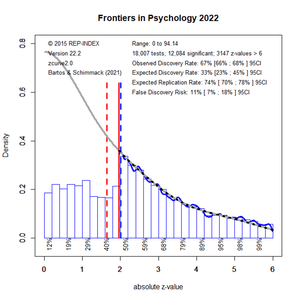


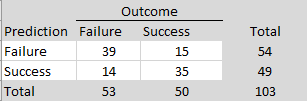


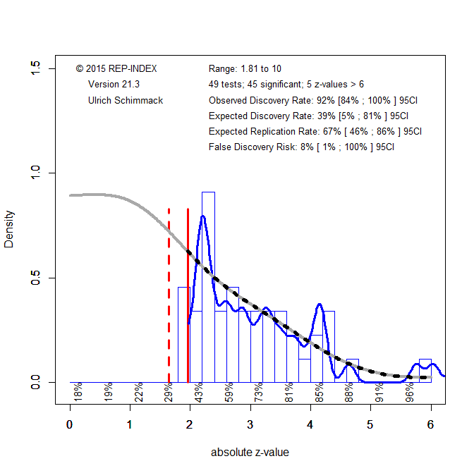


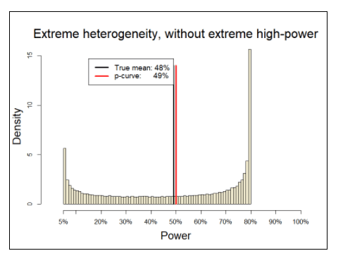


