How Science Should Work

Lay people, undergraduate students, and textbook authors have a simple model of science. Researchers develop theories that explain observable phenomena. These theories are based on exploratory research or deduced from existing theories. Based on a theory, researchers make novel predictions that can be subjected to empirical tests. The gold-standard for an empirical test is an experiment, but when experiments are impractical, quasi-experiments or correlational designs may be used. The minimal design examines whether two variables are related to each other. In an experiment, a relation exists when an experimentally created variation produces variation in observations on a variable of interest. In a correlational study, a relation exists when two variables covary with each other. When empirical results show the expected covariation, the results are considered supportive of a theory and the theory lives another day. When the expected covariation is not observed, the theory is challenged. If repeated attempts fail to show the expected effect, researchers start developing a new theory that is more consistent with the existing evidence. In this model of science, all scientists are only motivated by the goal to build a theory that is most consistent with a robust set of empirical findings.

The Challenge of Probabilistic Predictions and Findings

I distinguish two types of science; the distinction maps onto the distinction between hard and soft sciences, but I think the key difference between the two types of science is whether theories are used to test deterministic relationships (i.e., relationships that hold in virtually every test of the phenomenon) and probabilistic relationships, where a phenomenon may be observed only some of the time. An example of deterministic science is chemistry where the combination of oxygen and hydrogen leads to an explosion and water, when hydrogen and oxygen atoms combine to form H₂0. An example, of probabilistic science is a classic memory experiment where more recent information is more likely to be remembered than more remote information, but memory is not deterministic and it is possible that remote information is sometimes remembered better than recent information.   A unique challenge for probabilistic science is to interpret empirical evidence because it is possible to make two errors in the interpretation of empirical results. These errors are called type-I and type-II errors.

Type-I errors refer to the error that the data show a theoretically predicted result when the prediction is false.

Type-II errors refer to the error that the data do not show a theoretically predicted result when the prediction is correct.

There are many reasons why a particular study may produce misleading results. Most prominently, a study may have failed to control (experimentally or statistically) for confounding factors. Another reason could be that a manipulation failed or a measure failed to measure the intended construct. Aside from these practical problems in conducting an empirical study, type-I and type-II errors can still emerge even in the most carefully conducted study with perfect measures. The reason is that empirical results in tests of probabilistic hypothesis are influenced by factors that are not under the control of the experimenter. These causal factors are sometimes called random error, sampling error, or random sampling error. The main purpose of inferential statistics is to deal with type-I and type-II errors that are caused by random error. It is also possible to conduct statistical analysis without drawing conclusions from the results. These statistics are often called descriptive statistics. For example, it is possible to compute and report the mean and standard deviation of a measure, the mean difference between two groups, or the correlation between two variables in a sample. As long as these results are merely reported they simply describe an empirical fact. They also do not test a theoretical hypothesis because scientific theories cannot make predictions about empirical results in a specific sample. Type-I or Type-II errors occur when the empirical results are used to draw inferences about results in future studies, in the population, or about the truth of theoretical predictions.

Three Approaches to the Problem of Probabilistic Science

In the world of probabilities, there is no certainty, but there are different degrees of uncertainty. As the strength of empirical evidence increases, it becomes less likely that researchers make type-I or type-II errors.   The main aim of inferential statistics is to provide objective and quantitative information about the probability that empirical data provide the correct information about the hypothesis; that is to avoid making a type-I or type-II error.

Statisticians have developed three schools of thought: Fisherian, Neyman-Pearson, and Bayesian statistics. The problem is that contemporary proponents of these approaches are still fighting about the right approach. As a prominent statistician noted, “the effect on statistics of having three (actually more) warring factions… has not been good for our professional image” (Berger, 2003, p. 4). He goes on to note that statisticians have failed to make “a concerted professional effort to provide the scientific world with a unified testing methodology.”

For applied statisticians the distinction between Fisher and Neyman-Pearson is of relatively little practical concern because both approaches rely on the null-hypothesis and p-values. Statistics textbook often do present a hybrid model of both approaches. The Fisherian approach is to treat p-values as a measure of the strength of evidence against the null-hypothesis. As p-values approach zero, it becomes less and less likely that the null-hypothesis is true. For example, imagine a researcher computes the correlation between height and weight in a sample of N = 10 participants. The correlation is r = .50. Given the small sample size, this extreme deviation from the null-hypothesis could still have occurred by chance. As the sample size increases, random factors can produce only smaller and smaller deviations from zero and an observed correlation of r = .50 becomes less and less likely to have occurred as a result of random sampling error (oversampling tall and heavy participants and undersampling short and lightweight).

The main problem for Fisher’s approach is that it provides no guidelines about the size of a p-value that should be used to reject the null-hypothesis (there is no correlation) and therewith confirm the alternative (there is a correlation). Thus, p-values provide a quantitative measure of evidence against the null-hypothesis, but they do not provide a decision rule how strong the evidence should be to conclude that the null-hypothesis is false. As such, one might argue that Fisher’s approach is not an inferential statistical approach because it does not spell out how researchers should interpret p-values. Without a decision rule, a p-value is just an objective statistic like a sample mean or standard deviation.

Neyman-Pearson solved the problem of inference by introducing a criterion value. The most common criterion value is p = .05. When the strength of the evidence against the null-hypothesis leads to a p-value less than .05, the null-hypothesis is rejected. When the p-value is above the criterion, the null-hypothesis is accepted. According to Berger (2003), Neyman-Pearson also advocated to compute and report type-I and type-II error probabilities. Evidently, this suggestion has not been adopted in applied research, especially with regard to type-II error probabilities. The main reason for not adopting Neyman-Pearson’s recommendation is that the type-II error rate depends on an a priori assumption about the size of an effect. However, many hypothesis in the probabilities sciences make only diffuse, qualitative predictions (e.g., height will be positively correlated with weight, but the correlation may range anywhere from r = .1 to .8). Applied researchers saw little value in computing type-II error rates that are based on subjective assumptions about the strength of an effect. Instead, they adopted the criterion approach by Neyman-Pearson, but they used the criterion only to make the decision that the null-hypothesis is false when the evidence was strong enough to reject the null-hypothesis (p < .05). In contrast, when the evidence was not strong enough to reject the null-hypothesis, the results were considered inconclusive. The null-hypothesis could be true or the results were a type-II error. It was not important to determine whether the null-hypothesis was true or not because researchers were mainly interested in demonstrating causal relationships (a drug is effective) than in showing that something does not have an effect (a drug is not effective). By avoiding to rule in favor of the null-hypothesis, researchers could never make a type-II error in the classical sense that they falsely accepted the null-hypothesis. In this context, the term type-II error assumed a new meaning. A type-II error now meant that the study had insufficient statistical power to demonstrate that the null-hypothesis was false. A study with more statistical power might be able to produce a p-value less than .05 and demonstrate that the null-hypothesis is false.

The appeal of the hybrid approach was that the criterion provided meaningful information about the type-I error and that the type-II error rate was zero because results were never interpreted as favoring the null-hypothesis. The problem of this approach is that it can never lead to the conclusion that an effect is not present. For example, it is only possible to demonstrate gender differences, but it is never possible to demonstrate that men and women do not differ from each other. The main problem with this one-sided testing approach was that non-significant results seemed unimportant because they were inconclusive and it seemed more important to report conclusive, significant results than inconclusive and insignificant results. However, if only significant results are reported, it is no longer clear how many of these significant results might be type-I errors (Sterling, 1959). If only significant results are reported, the literature will be biased and can contain an undetermined amount of type-I errors (false evidence for an effect when the null-hypothesis is true). However, this is not a problem of p-values. It is a problem of not reporting studies that failed to provide support for a hypothesis, which is needed to reveal type-I errors. As type-I errors would occur only at a rate of 1 out of 20, honest reporting of all studies would quickly reveal which significant results are type-I errors.

Bayesian Statistics

The Bayesian tradition is not a unified approach to statistical inference. The main common element of Bayesian statistics is to criticize p-values because they do not provide information about the probability that a hypothesis is true; p(H1|D). Bayesians argue that empirical scientists misinterpret p-values as estimates of the probability that a hypothesis is true, when they quantify merely the probability that the data could have been produced without an effect. The main aim of Bayesian statistics is to use the Bayes Theorem to obtain an estimate of p(H1|D) from the empirically observed data.

One piece of information is the probability of an empirical observed statistic when the null-hypothesis is true, p(D|H0). This probability is closely related to p-values. Whereas the Bayesian p(D|H0) is the probability of obtaining a particular test statistic (e.g., a z-score of 1.65), p-values quantify the probability of obtaining a test statistic greater (one-sided) than the observed test statistic (p[z > 1.65] = .05) [for the two-sided case, p[abs(z) = 1.96] = .05]

The problem for estimating the probability that the hypothesis is true given an empirical result depends on three more probabilities that are unrelated to the observed data, namely the probability that the hypothesis is true, P(H0), the probability that the alternative hypothesis is true, p(H1), and the probability that the data would have been observed if the alternative hypothesis is true, p(D|H1). One approach to the problem of three unknowns is to use prior knowledge or empirical data to estimate these parameters. However, the problem for many empirical studies is that there is very little reliable a priori information that can be used to estimate these parameters.

A group of Bayesian psychologists has advocated an objective Bayesian approach to deal with problem of unknown parameters in Bayes’ Theorem (Wagenmakers et al., 2011). To deal with the problem that p(H1|D) is unknown, the authors advocate using a default a priori probability distribution of effect sizes. The next step is to compute the ratio of p(H0|D) and p(H1|D). This ratio is called the Bayes-Factor. The following formula shows that the probability of the null-hypothesis being true given the data, p(H0|D), increases as the Bayes-Factor, p(D|H0)/p(D|H1) increases. Similarly, the probability of the alternative hypothesis given the data, p(H1|D) increases as the Bayes-Factor decreases. To quantify these probabilities, one would need to make assumptions about p(H0) and p(H1), but even without making assumptions about these probabilities, it is clear that the ratio of p(H0|D)/p(H1|D) is proportional to p(D|H0)/p(D|H1).

Bayes-Factors have two limitations. First, like p-values, Bayes-Factors alone are insufficient for inferential statistics because they only quantify the relative evidence in favor of two competing hypotheses. It is not clear at which point the results of a study should be interpreted as evidence for one of the two hypotheses. For example, is a Bayes-Factor of 1.1, 2.5, 3, 10, or 100 sufficient to conclude that the null-hypothesis is true? The second problem is that the default function may not adequately characterize the alternative hypothesis. In this regard, Bayesian statistics have the same problem as Neyman-Pearson’s approach that required making a priori assumptions about the effect size in order to compute type-II error rates.  In Bayesian statistic the a priori distribution of effect sizes influences the Bayes-Factor.

In response to the first problem, Bayesians often use conventional criterion values that are used to make decisions based on empirical data. Commonly used criterion values are a Bayes-Factor of 3 or 10. A decision rule is clearly implemented in Bayesian studies with optional stopping where a Bayes-Factor of 10 or greater is used to justify terminating a study early. Bayes-Factors with a decision criterion create a new problem in that it is now possible to obtain inconclusive results and results that favor the null-hypothesis. As a result, there are now two types of type-II errors. Some type-II errors occur when the BF meets the criterion to accept the null-hypothesis when the null-hypothesis is false. Other type-II errors occur when the null-hypothesis is false and the data are inconclusive.

So far, Bayesian statisticians have not examined type-II error rates with the argument that Bayes-Factors do not require researchers to make decisions. However, without clear decision rules, Bayes-Factors are not very appealing to applied scientists because researchers, reviewers, editors, and readers need some rational criterion to make decisions about publication and planning of future studies. The best way to provide this information would be to examine how often Bayes-Factors of a certain magnitude lead to false conclusions; that is, to determine the type-I and type-II(a,b) error rates that are associated with a Bayes-Factor of a certain magnitude. This question has not been systematically examined.

The Bayesian Default T-Test

As noted above, there is no unified Bayesian approach to statistical inference. Thus, it is impossible to make general statements about Bayesian statistics. Here I focus on the statistical properties of the default Bayesian t-test (Rouder, Speckman, Sun, Morey, & Iverson, 2009). Most prominently, this test was used to demonstrate the superiority of Bayes-Factors over p-values with Bem’s (2011) controversial set of studies that seemed to support extrasensory perception.

The authors provide an R-package with a function that computes Bayes-Factors based on the observed t-statistic and degrees of freedom. It is noteworthy that the Bayes-Factor is fully determined by the t-value, the degrees of freedom, and a default scaling parameter for the prior distribution. As t-values and df are also used to compute p-values, Bayes-Factors and p-values are related to each other.  The main difference is that p-values have a constant meaning for different sample sizes. That is, p = .04 has the same meaning in studies with N = 10, 100, or 1000 participants. However, Bayes-Factors for the same t-value changes as a function of sample size.

“With smaller sample sizes that are insufficient to differentiate between approximate and exact invariances, the Bayes factors allows researchers to gain evidence for the null. This evidence may be interpreted as support for at least an approximate invariance. In very large samples, however, the Bayes factor allows for the discovery of small perturbations that negate the existence of an exact invariance.” (Rouder et al., 2009, p 233).

This means that the same population effect size can produce three different outcomes depending on sample size; it may show evidence in favor of the null-hypothesis with a small sample size, it may show inconclusive results with a moderate sample size, and it may show evidence for the alternative hypothesis with a large sample size.

The ability to compute Bayes-Factors and p-values from t-values also implies that for a fixed sample size, p-values can be directly transformed into Bayes-Factors and vice versa. This makes it easy to directly compare the inferences that can be drawn from observed t-values for different p-values and Bayes-Factors.

The simulations used the default setting of a Cauchi distribution with a scale parameter of .707.

The x-axis shows potential effect sizes. The y-axis shows the weight attached to different effect sizes. The Cauchy distribution is centered over zero, giving the highest probability to an effect size of d = 0. As effect sizes increase weights decrease. However, even effect sizes greater than d = .8 (strong effect, Cohen, 1988) still have notable weights and the distribution includes effect sizes above d = 2. It is important to keep in mind that Bayes-Factors express the relative strength of evidence for or against the null-hypothesis relative to the weighted average effect size implied by the default function. Thus, it is possible that a Bayes-Factor favors the null-hypothesis if the population effect size is small because a small effect size is inconsistent with a prior distribution that considers strong effect sizes as a possible outcome.

The next figure shows Bayes-Factors as a function of p-values for an independent group t-test with n = 50 per condition. The black line shows the Bayes-Factor for H1 over H0. The red line shows the Bayes-Factor for H0 over H1. I show both ratios because I find it easier to compare Bayes-Factors greater than 1 than Bayes-Factors less than 1. The two lines cross when BF = 1, which is the point where the data favor both hypothesis equally.

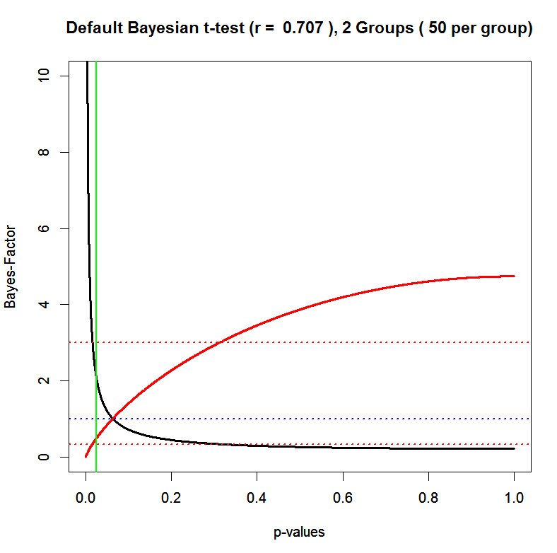
The graph shows the monotonic relationship between Bayes-Factors and p-values. As p-values decrease BF10 (favor H1 over H0, black) increases. As p-values increase, BF01-values (favor H0 over H1, red) also increase. However, the shapes of the two curves are rather different. As p-values decrease, the black line stays flat for a long time. As p-values are around p = .2, the curve goes up. It reaches a value of 3 just below a p-value of .05 (marked by the green line) and then increases quickly. This graph suggests that a Bayes-Factor of 3 corresponds roughly to a p-value of .05. A Bayes-Factor of 10 would correspond to a more stringent p-value. The red curve has a different shape. Starting from the left, it rises rather quickly and then slows down as p-values move towards 1. BF01 cross the red dotted line marking BF = 3 at around p = .3, but it never reaches a factor of 10 in favor of the null-hypothesis. Thus, using a criterion of BF = 3, p-values higher than .3 would be interpreted as evidence in favor of the null-hypothesis.

The next figure shows the same plot for different sample sizes.

The graph shows how the Bayes-Factor of H0 over H1 (red line) increases as a function of sample size. It also reaches the critical value of BF = 3 earlier and earlier. With n = 1000 in each group (total N = 2000) the default Bayesian test is very likely to produce strong evidence in favor of either H1 or H0.

The responsiveness of BF01 to sample size makes sense. As sample size increases, statistical power to detect smaller and smaller effects also increases. In the limit a study with an infinite sample size has 100% power. That means, when the whole population has been studied and the effect size is zero, the null-hypothesis has been proven. However, even the smallest deviation from zero in the population will refute the null-hypothesis because sampling error is zero and the observed effect size is different from zero.

The graph also shows that Bayes-Factors and p-values provide approximately the same information when H1 is true. Statistical decisions based on BF10 or p-values lead to the same conclusion for matching criterion values. The standard criterion of p = .05 corresponds approximately to BF10 = 3 and BF10 = 10 corresponds roughly to p = .005. Thus, Bayes-Factors are not less likely to produce type-I errors than p-values because they reflect the same information, namely how unlikely it is that the deviation from zero in the sample is simply due to chance.

The main difference between Bayes-Factors and p-values arises in the interpretation of non-significant results (p > .05, BF10 < 3). The classic Neyman-Pearson approach would treat all non-significant results as evidence for the null-hypothesis, but would also try to quantify the type-II error rate (Berger, 2003). The Fisher-Neyman-Pearson hybrid approach treats all non-significant results as inconclusive and never decides in favor of the null-hypothesis. The default Bayesian t-tests distinguishes between inconclusive results and those that favor the null-hypothesis. To distinguish between these two conclusions, it is necessary to postulate a criterion value. Using the same criterion that is used to rule in favor of the alternative hypothesis (p = .05 ~ BF10 = 3), a BF01 > 3 is a reasonable criterion to decide in favor of the null-hypothesis. Moreover, a more stringent criterion would not be useful in small samples, because BF01 can never reach values of 10 or higher. Thus, in small samples, the conclusion would always be the same as in the standard approach that treats all non-significant results as inconclusive.

Power, Type I, and Type-II Error rates of the default Bayesian t-test with BF=3 as criterion value

As demonstrated in the previous section, the results of a default Bayesian t-test depend on the amount of sampling error, which is fully determined by sample size in a between-subject design. The previous results also showed that the default Bayesian t-test has modest power to rule in favor of the null-hypothesis in small samples.

For the first simulation, I used a sample size of n = 50 per group (N = 100). The reason is that Wagenmakers and colleagues have conducted several pre-registered replication studies with a stopping rule when sample size reaches N= 100. The simulation examines how often a default t-test with 100 participants can correctly identify the null-hypothesis when the null-hypothesis is true. The criterion value was set to BF01 = 3. As the previous graph showed, this implies that any observed p-value of approximately p = .30 to 1 is considered to be evidence in favor of the null-hypothesis. The simulation with 10,000 t-tests produced 6,927 BF01s greater than 3. This result is to be expected because p-values follow a uniform distribution when the null-hypothesis is true. Therefore, the p-value that corresponds to BF01 = 3 determines the rate of decisions in favor of null. With p = .30 as the criterion value that corresponds to BF01 = 3, 70% of the p-values are in the range from .30 to 1. 70% power may be deemed sufficient.

The next question is how the default Bayesian t-test behaves when the null-hypothesis is false. The answer to this question depends on the actual effect size. I conducted three simulation studies. The first simulation examined effect sizes in the moderate to large range (d = .5 to .8). Effect sizes were uniformly distributed. With a uniform distribution of effect sizes, true power ranges from 70% to 97% with an average power of 87% for the traditional criterion value of p = .05 (two-tailed). Consistent with this power analysis, the simulation produced 8704 significant results. Using the BF10 = 3 criterion, the simulation produced 7405 results that favored the alternative hypothesis with a Bayes-Factor greater than 3. The power is slightly lower than for p=.05 because BF = 3 is a slightly stricter criterion. More important, the power of the test to show support for the alternative is about equal to the power to support the null-hypothesis; 74% vs. 70%, respectively.

The next simulation examined effect sizes in the small to moderate range (d = .2 to .5). Power ranges from 17% to 70% with an average power of 42%. Consistent with this prediction, the simulation study with 10,000 t-tests produced 4072 significant results with p < .05 as criterion. With the somewhat stricter criterion of BF = 3, it produced only 2,434 results that favored the alternative hypothesis with BF > 3. More problematic is the finding that it favored the null-hypothesis (BF01 > 3) nearly as often, namely 2405 times. This means, that in a between-subject design with 100 participants and a criterion-value of BF = 3, the study has about 25% power to demonstrate that an effect is present, it will produce inconclusive results in 50% of all cases, and it will falsely support the null-hypothesis in 25% of all cases.

Things get even worse when the true effect size is very small (d > 0, d < .2). In this case, power ranges from just over .05, the type-I error rate, to just under 17% for d = .2. The average power is just 8%. Consistent with this prediction, the simulation produced only 823 out of 10,000 significant results with the traditional p = .05 criterion. The stricter BF = 3 criterion favored the alternative hypothesis in only 289 out of 10,000 cases with a BF greater than 3. However, BF01 exceeded a value of 3 in 6201 cases. The remaining 3519 cases produced inconclusive results. In this case, the Bayes-Factor favored the null-hypothesis when it was actually false. The rate of false decisions in favor of the null-hypothesis is nearly as high as the power of the test to correctly identify the null-hypothesis (62% vs. 70%).

The previous analyses indicate that Bayes-Factors produce meaningful results when power to detect an effect is high, but that Bayes-Factors are at risk to falsely favor the null-hypothesis when power is low. The next simulation directly examined the relationship between power and Bayes-Factors. The simulation used effect sizes in the range from d = .001 to d = 8 with N = 100. This creates a range of power from 5 to 97% with an average power of 51%.

In this figure, red data points show BF01 and blue data points show BF10. The right side of the figure shows that high-powered studies provide meaningful information about the population effect size as BF10 tend to be above the criterion value of 3 and BF01 are very rarely above the criterion value of 3. In contrast, on the left side, the results are misleading because most of the blue data points are below the criterion value of 3 and many BF01 data points are above the criterion value of BF = 3.

What about the probability of the data when the default alternative hypothesis is true?

A Bayes-Factor is defined as the ratio of two probabilities, the probability of the data when the null-hypothesis is true and the probability of the data when the null-hypothesis is false.  As such, Bayes-Factors combine information about two hypotheses, but it might be informative to examine each hypothesis separately. What is the probability of the data when the null-hypothesis is true and what is the probability of the data when the alternative hypothesis is true? To examine this, I computed p(D|H1) by dividing the p-values by BF01 for t-values in the range from 0 to 5.

BF01 = p(D|H0) / p(D|H1)   =>    p(D|H1) = BF01 * p(D|H0)

As Bayes-Factors are sensitive to sample size (degrees of freedom), I repeated the analysis with N = 40 (n = 20), N = 100 (n = 50), and N = 200 (n = 100).

The most noteworthy aspect of the figure is that p-values (the black line, p(D|H0)), are much more sensitive to changes in t-values than the probabilities of the data given the alternative hypothesis (yellow N=40, orange N=100, red N=200). The reason is the diffuse nature of the alternative hypothesis. It always includes a hypothesis that predicts the test-statistic, but it also includes many other hypotheses that make other predictions. This makes the relationship between the observed test-statistic, t, and the probability of t given the diffuse alternative hypothesis dull. The figure also shows that p(D|H0) and p(D|H1) both decrease monotonically as t-values increase. The reason is that the default prior distribution has its mode over 0. Thus, it also predicts that an effect size of 0 is the most likely outcome. It is therefore not a real alternative hypothesis that predicts an alternative effect size. It merely is a function that has a more muted relationship to the observed t-values. As a result, it is less compatible with low t-values and more compatible with high t-values than the steeper function for the point-null hypotheses.

Do we need Bayes-Factors to Provide Evidence in Favor of the Null-Hypothesis?

A common criticism of p-values is that they can only provide evidence against the null-hypothesis, but that they can never demonstrate that the null-hypothesis is true. Bayes-Factors have been advocated as a solution to this alleged problem. However, most researchers are not interested in testing the null-hypothesis. They want to demonstrate that a relationship exists. There are many reasons why a study may fail to produce the expected effect. However, when the predicted effect emerges, p-values can be used to rule out (with a fixed error probability) that the effect emerged simply as a result of chance alone.

Nevertheless, non-Bayesian statistics could also be used to examine whether a null-hypothesis is true without the need to construct diffuse priors or to compare the null-hypothesis to an alternative hypothesis. The approach is so simple that it is hard to find sources that explain it. Let’s assume that a researcher wants to test the null-hypothesis that Bayesian statisticians and other statisticians are equally intelligent. The researcher recruits 20 Bayesian statisticians and 20 frequentist statisticians and administers an IQ test. The Bayesian statisticians have an average IQ of 130 points. The frequentists have an average IQ of 120 points. The standard deviation of IQ scores on this IQ test is 15 points. Moreover, it has been shown that IQ scores are approximately normally distributed. Thus, sampling error is defined as 15 * (2 / sqrt(40)) = 4.7 ~ 5. The figure below shows the distribution of difference scores under the assumption that the null-hypothesis is true. The red lines show the 95% confidence interval. A 5 point difference is well within the 95% confidence interval. Thus, the result is consistent with the null-hypothesis that there is no difference in intelligence between the two groups. Of course, a 5 point difference is one-third of a standard deviation, but the sample size is simply too small to infer from the data that the null-hypothesis is false.

A more stringent test of the null-hypothesis would require a larger sample. A frequentist researcher conducts a power analysis and assumes that only a 5 point difference or more would be meaningful. She conducts a power analysis and finds that a study with 143 participants in each group (N = 286) is needed to have 80% power to show a difference of 5 points or more. A non-significant result would suggest that the difference is smaller or that a type-II error occurred with a 20% probability. The study yields a mean of 128 for frequentists and 125 for Bayesians. The 3 point difference is not significant. As a result, the data support the null-hypothesis that Bayesians and Frequentists do not differ in intelligence by more than 5 points. A more stringent test of equality or invariance would require an even larger sample. There is no magic Bayesian bullet that can test a precise null-hypothesis in small samples.

Ignoring Small Effects is Rational: Parsimony and Occam’s Razor

Another common criticism of p-values is that they are prejudice against the null-hypothesis because it is always possible to get a significant result simply by increasing sample size. With N = 1,000,000, a study has 95% power to detect even an effect size of d = .007. The argument is that it is meaningless to demonstrate significance in smaller samples, if it is certain that significance can always be obtained in a larger sample. The argument is flawed because it is simply not true that p-values will eventually produce a significant result when sample sizes increase. P-values will only produce significant results when a true effect exists. When the null-hypothesis is true an honest test of the hypothesis will only produce as many significant results as the type-I error criterion specifies. Moreover, Bayes-Factors are no solution to this problem. When a true effect exists, they will also favor the alternative hypothesis no matter how small the effect is and when sample sizes are large enough to have sufficient power. The only difference is that Bayes-Factors may falsely accept the null-hypothesis in smaller samples.

The more interesting argument against p-value is not that significant results in large studies are type-I errors, but that these results are practically meaningless. To make this point, statistics books often distinguish statistical significance and practical significance and warn that statistically significant results in large samples may have little practical significance. This warning was useful in the past when researchers would only report p-values (e.g., women have higher verbal intelligence than men, p < .05). The p-value says nothing about the size of the effect. When only the p-value is available, it makes sense to assume that significant results in smaller samples are larger because only large effects can be significant in these samples. However, large effects can also be significant in large samples and large effects in small studies can be inflated by sampling error. Thus, the notion of practical significance is outdated and should be replaced by questions about effect sizes. Neither p-values nor Bayes-Factors provide information about the size of the effect or the practical implications of a finding.

How can p-values be useful when there is clear evidence of a replication crisis?

Bem (2011) conducted 10 studies to demonstrate experimental evidence for anomalous retroactive influences on cognition and affect. His article reports 9 significant results and one marginally significant result. Subsequent studies have failed to replicate this finding. Wagenmakers et al. (2011) used Bem’s results as an example to highlight the advantages of Bayesian statistics. The logic was that p-values are flawed and that Bayes-Factors would have revealed that Bem’s (2011) evidence was weak. There are several problems with Wagenmaker et al.’s (2011) Bayesian analysis of Bem’s data.

First, the reported results differ from the default Bayesian-test implemented on Dr. Rouder’s website (http://pcl.missouri.edu/bf-one-sample). The reason is that Bayes-Factors depend on a scaling factor of the Cauchy distribution. Wagenmakers et al. (2011) used a scaling factor of 1, whereas the online app used .707 as the default. The choice of a scaling parameter gives some degrees of freedom to researchers. Researchers who favor the null-hypothesis can choose a larger scaling factor which makes the alternative hypothesis more extreme and easier to reject with small effects. Smaller scaling factors make the Cauchy-distribution narrower and it is easier to show evidence in favor of the alternative hypothesis with smaller effects. The behavior of Bayes-Factors for different scaling parameters is illustrated in Table 1 with Bem’s data.

 

Experiment 7 is highlighted because Bem (2011) already interpreted the non-significant result in this study as evidence that the effect disappears with supraliminal stimuli; that is, visible stimuli. The Bayes-Factor would support Bem’s (2011) conclusion that Experiment 7 shows evidence that the effect does not exist under this condition. The other studies essentially produced inconclusive Bayes-Factors, especially for the online default-setting with a scaling factor of .707. The only study that produced clear evidence for ESP was experiment 9. This study had the smallest sample size (N = 50), but a large effect size that was twice the effect size in the other studies. Of course, this difference is not reliable due to the small sample size, but it highlights how sensitive Bayes-Factors are to sampling error in small samples.

Another important feature of the Bayesian default t-test is that it centers the alternative hypothesis over 0. That is, it assigns the highest probability to the null-hypothesis, which is somewhat odd as the alternative hypothesis states that an effect should be present. The justification for this default setting is that the actual magnitude of the effect is unknown. However, it is typically possible to formulate an alternative hypothesis that allows for uncertainty, while predicting that the most likely outcome is a non-null effect size. This is especially true when previous studies provide some information about expected effect sizes. In fact, Bem (2011) explicitly planned his study with the expectation that the true effect size is small, d ~ .2. Moreover, it was demonstrated above that the default t-test is biased against small effects. Thus, the default Bayesian t-test with a scaling factor of 1 does not provide a fair test of Bem’s hypothesis against the null-hypothesis.

It is possible to use the default t-test to examine how consistent the data are with Bem’s (2011) a priori prediction that the effect size is d = .2. To do this, the null-hypothesis can be formulated as d = .2 and t-values can be computed as deviations from a population parameter d = .2. In this case, the null-hypothesis presents Bem’s (2011) a priori prediction and the alternative prediction is that observed effect sizes will deviated from this prediction because the effect is smaller (or larger). The next table shows the results for the Bayesian t-test that tests H0: d = .2 against a diffuse alternative H1: Cauchy-distribution centered over d = .2. Results are presented as BF01 so that Bayes-Factors greater than 3 indicate support for Bem’s (2011) prediction.

The Bayes-Factor supports Bem’s prediction in all tests. Choosing a wider alternative this time provides even stronger support for Bem’s prediction because the data are very consistent with the point prediction of a small effect size, d = .2. Moreover, even Experiment 7 now shows support for the hypothesis because an effect size of d = .09 is still more likely to have occurred when the effect size is d = .2 than for a wide-range of other effect sizes. Finally, Experiment 9 now shows the weakest support for the hypothesis. The reason is that Bem used only 50 participants in this study and the effect size was unusually large. This produced a low p-value in a test against zero, but it also produced the largest deviation from the a priori effect size of d = .2. However, this is to be expected in a small sample with large sampling error. Thus, the results are still supportive, but the evidence is rather weak compared to studies with larger samples and effect sizes close to d = 2.

The results demonstrate that Bayes-Factors cannot be interpreted as evidence for or against a specific hypothesis. They are influenced by the choice of the hypotheses that are being tested. In contrast, p-values have a consistent meaning. They quantify how probable it is that random sampling error alone could have produced a deviation between an observed sample parameter and a postulated population parameter. Bayesians have argued that this information is irrelevant and does not provide useful information for the testing of hypotheses. Although it is true that p-values do not quantify the probability that a hypothesis is true when significant results were observed, Bayes-Factors also do not provide this information. Moreover, Bayes-Factors are simply a ratio of two probabilities that compare two hypotheses against each other, but usually only one of the hypotheses is of theoretical interest. Without a principled and transparent approach to the formulation of alternative hypotheses, Bayes-Factors have no meaning and will change depending on different choices of the alternatives. The default approach aims to solve this by using a one-size-fits-all solution to the selection of priors. However, inappropriate priors will lead to invalid results and the diffuse Cauchy-distribution never fits any a priori theory.

 Conclusion

Statisticians have been fighting for supremacy for decades. Like civilians in a war, empirical scientists have suffered from this war because they have been bombarded by propaganda and they have been criticized that they misunderstand statistics or use the wrong statistics. In reality, the statistical approaches are all related to each other and they all rely on the ratio of the observed effect sizes to sampling error (i.e, the signal to noise ratio) to draw inferences from observed data about hypotheses. Moreover, all statistical inferences are subject to the rule that studies with less sampling error provide more robust empirical evidence than studies with more sampling error. The biggest challenge for empirical researchers is to optimize the allocation of resources so that each study has high statistical power to produce a significant result when an effect exists. With high statistical power to detect an effect, p-values are likely to be small (50% chance to get a p-value of .005 or lower with 80% power) and Bayes-Factors and p-values provide virtually the same information for matching criterion values, when an effect is present. High power also implies a relative low frequency of type-II errors, which makes it more likely that a non-significant result occurred because the hypothesis is wrong.  Thus, planning studies with high power is important no matter whether data are analyzed with Frequentist or Bayesian statistics.

Studies that aim to demonstrate the lack of an effect or an invariance (there is no difference in intelligence between Bayesian and frequentist statisticians) need large samples to demonstrate invariance or have to accept that there is a high probability that a larger study would find a reliable difference. Bayes-Factors do not provide a magical tool to provide strong support for the null-hypothesis in small samples. In small samples Bayes-Factors can falsely favor the null-hypothesis even when effect sizes are in the moderate to large range.

In conclusion, like p-values, Bayes-Factors are not wrong.  They are mathematically defined entities.  However, when p-values or Bayes-Factors are used by empirical scientists to interpret their data, it is important that the numeric results are interpreted properly.  False interpretation of Bayes-Factors is just as problematic as false interpretation of p-values.  Hopefully, this blog post provided some useful information about Bayes-Factors and their relationship to p-values.